In this tutorial, 2D and 3D data will be combined in an ArcGIS Pro Local Scene to visualize the topography, imagery, and cultural features of a region in the state of Washington. Mapping and modeling in 3D makes it easier to understand and communicate the effects of natural events such as volcanic mudflow (lahar).
What you will need
- Access to an ArcGIS Pro license
- Sample dataset downloaded from ArcUser website
- Unzipping utilty
For this tutorial and in the three previous ones in this series, the area mapped was the site of an international emergency planning and response exercise that was conducted in November 2017. That exercise, the fifth Canada-United States Enhanced Resiliency Experiment (CAUSE V) exercise, was conducted in Whatcom County, Washington, and southern British Columbia, Canada.
The data captured during that exercise has been the basis for four tutorials in ArcUser. The first tutorial, “Modeling Volcanic Mudflow Travel Time with ArcGIS Pro and ArcGIS Network Analyst,” appeared in the Fall 2017 issue of ArcUser. It introduced a special use of ArcGIS Network Analyst, an ArcGIS Pro extension, to model lahar as it ran down the Nooksack River, through several communities, and into Puget Sound as the result of a hypothetical seismic event—the crater collapse on Mount Baker.
The second tutorial, “Georeferencing Drone-Captured Imagery,” in the Winter 2018 issue, showed a simple imagery georeferencing workflow that imported an ArcMap document (MXD) into ArcGIS Pro. In that exercise, two images were georeferenced by interactively connecting the ground control targets on the raster with vector control points.
“Test Georeferencing Transformations,” which ran in the Spring 2018 issue, showed how to georeference an image by importing a file containing ground control points and explored the effects of all the transformations available in ArcGIS Pro.
“Mapping and Modeling Lidar Data with ArcGIS Pro,” the most recent tutorial, which appeared the summer 2018 issue of ArcUser, showed how to compare bare earth and first return lidar rasters to explore natural and cultural features in ArcGIS Pro.
Monitoring the Exercise with Drones
One of the critical tests conducted during CAUSE V was capturing high-resolution and real-time data transmitted from the field to the CAUSE V Emergency Operations Center. On the second day of the exercise, drones were deployed along the Nooksack River to assess, capture, and relay event status to headquarters for follow-up mapping, incident management, and response planning.
One of those drones, Drone 4, was stationed on the north side of the Nooksack River, just above the Washington State Route 544 (WA Hwy) bridge. This bridge bisects the town of Everson and is the only means of crossing the Nooksack River at that point. Drone 4 was assigned to assess the bridge’s condition, monitor traffic flow, and identify threats to the structure and the surrounding community. The drone was also tasked with monitoring anticipated debris flow from the Nooksack River, over a low divide into Johnson Creek, and into the Sumas River, flowing toward Canada.
Getting Started
Although this exercise uses essentially the same data as was provided for the previous tutorial, use the sample dataset that accompanies the online version of this article. Several vector datasets have been modified and filtered to support 3D modeling, although the lidar data used to create hillshades, feature heights, and contours is unchanged. After you complete this tutorial, you could re-create those derivative products and add them to the final 3D scene.
Download the sample dataset, CAUSE_V_Drone_v21n4, for this tutorial from esri.com/arcuser and unzip it on a local machine. It should contain slightly more than 61 MB of data.
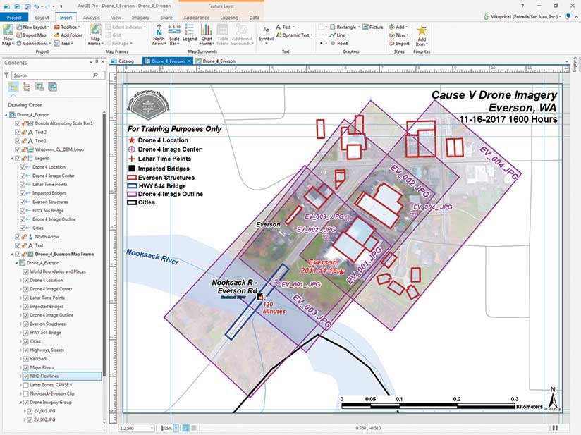
Start an ArcGIS Pro session, browse to CAUSE_V_Drone_v21n4\Drone_4_Everson and open the new Drone_4_Everson.aprx. [Do not open a project from a previous tutorial in this series.]
Drone_4_Everson is in ArcGIS Pro layout mode. It contains a new feature class, HWY 544 Bridge. Switch from layout to map view, open Bookmarks, and zoom to Everson 1:2,500.
All data layers posted in this map—except World Imagery and World Boundaries and Places—are projected in the same coordinate system—Zone 10 N, universal transverse Mercator (UTM) using the North American Datum 1983 (NAD83) and metric units.
Reviewing Vector and Raster Data
Click the tab to switch the view to map view. In the Contents pane, right-click the Everson Structures layer and open its attribute table. In the table, inspect the fields and note two numeric fields, Height_M and Elev_M. The attributes in these fields will be used to place structures and a bridge in 3D space. Close the attribute table.
Return to the Contents pane and open the attributes table for HWY 544 Bridge. This layer now displays a single polygon and has been separated from other polygons in the Everson Structures layer by applying a definition query. Notice that its height is zero and its elevation is 30.5 meters. Close the attribute table.
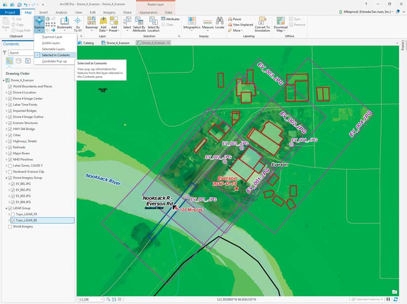
Scroll to the bottom of the Contents pane and make Topo_LiDAR_BE visible. This is the same bare earth lidar data that was used to create a hillshade and contours in the previous tutorial.
To better understand how this layer might behave in 3D, define a Pop-up (Identify) rule for a single Contents item by clicking the Map tab, then click the drop-down arrow at the bottom of the Explore tool and choose Selected in Contents. Return to the Contents pane, select Topo_LiDAR_BE, and click any area near the center of the HWY 544 Bridge (which is outlined in blue). The elevation value displayed in the pop-up should be 24 meters or less.
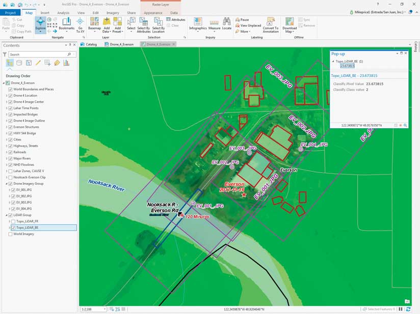
Click in adjacent areas to check other pixels in this bare earth raster to check the elevation values. As you click, you may notice that other visible raster layers may flash, but they are not selected, so no pop-up data is returned.
Return to the Contents pane, uncheck Topo_LiDAR_BE, make Topo_LiDAR_FR visible, and click on pixels in this layer located on the bridge. The elevation values on the bridge should be clustered around 30.8 meters. To query both bare earth and first return rasters, make them both visible and select both and click an area inside the HWY 544 Bridge polygon to display values from both rasters. In the next step, the Drone_4_Everson map will be converted to a 3D scene, and both lidar rasters will be used for data display and visualization. Save the project.
Everson in Three Dimensions
There are two viewing modes for scenes: global and local. Global is used for content that covers a large area and for which the curvature of the earth is an important element. Local is used for extents that are smaller and are in a projected coordinate system or for applications when the curvature of the earth isn’t needed.
Because this is a small area and it is in a projected coordinate system, convert this map to a Local Scene. Click the View tab and open the Catalog pane and expand the Maps item. Right-click Drone_4_Everson, open Convert, and choose To Local Scene.
Wait patiently as the 3D scene builds. Drone_4_Everson_3D appears on a tab to the right of the Drone_4_Everson map. Verify that Drone_4_Everson_3D is active.
Click the Map tab and click Bookmarks to see bookmarks for both 2D and 3D maps. Select the 3D Everson 1:2,500 bookmark. All four image outline polygons that will be used for georeferencing will be visible.
Displaying and Navigating in 3D
In the Contents pane, note the 3D layer group in Drone_4_Everson_3D does not contain any layers. As 2D objects are placed in 3D space, layers will be automatically generated and moved into the 3D group.
At the bottom of the Contents pane, in the Elevation Surfaces group layer, is a subgroup called Ground. This subgroup contains the WorldElevation3D/Terrain3D layer. This default surface, registered in World Geodetic System (WGS) 1984 Web Mercator (auxiliary sphere), initially posts the 2D vector and eventually raster data in 3D. Using this layer successfully requires a reasonably fast Internet connection.
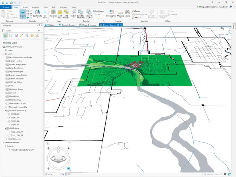
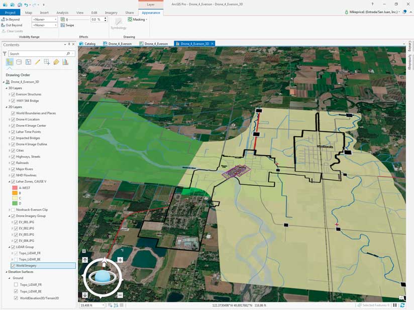
Click the 3D Everson 1:25,000 bookmark to zoom out to the full project extent. ArcGIS Pro Navigator appears in the lower left side of the scene. Even though the map still looks flat, the navigator can be used to explore Everson in 3D.
Click the up-facing caret in the navigator control’s upper-left corner to show the navigator in full control mode. Experiment with navigator. If you are not familiar with the navigator, read the ArcGIS Pro help for more information.
Adding Local Lidar Surfaces
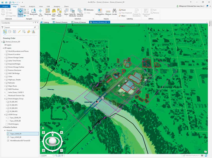
Use the 3D Everson 1:2,500 bookmark to zoom in. Angle the view point using navigator. Go to the bottom of the Contents pane. Under Elevation Surfaces, right-click the Ground subgroup. In the context menu, choose Add an Elevation Layer. Navigate to GDBFiles\UTM83Z10\Topo_LiDAR.gdb and add Topo_LiDAR_BE. Watch as the bare earth lidar raster loads and notice the increased resolution provided by the draped vectors.
Use the same process to add Topo_LiDAR_FR. Watch as the first return surface pushes vector data to higher elevations. Notice that all 2D vector feature classes are suspended on the highest visible ground elevation surface.
Initially, all vector data drapes on the WorldElevation3D ground surface. Now the forest canopy, approximate shape of structures, and the HWY 544 bridge are visible. Because these surfaces have one-meter pixels, the level of topographic detail is very high. Save the project.
Enhancing Vector Polygon Surfaces
In the Ground subgroup, turn off Topo_LiDAR_FR and WorldElevation3D, but leave Topo_LiDAR_BE on. Zoom in to show all image outlines.
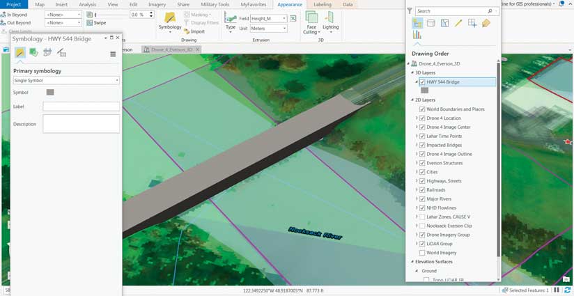
In the Contents pane, select HWY 544 Bridge and click the Appearance tab. In the Extrusion group, click the drop-down below Type and study the extrusion types. The default is None. The other choices are Min Height, Max Height, Base Height, and Absolute Height. Since the bridge is essentially flat, click Absolute Height to place it in 3D space.
In the Extrusion area, set the Field to Elev_M (to use the field values previously previewed in the attribute table for this layer) and confirm units as Meters. Zoom in to the bridge. Click Save to apply these updates. Notice that the bridge is now in the 3D Layers group.
The bridge symbology is a blue outline, which does not display well in 3D. Right-click the HWY 544 Bridge layer and select Symbology. In the Symbology pane, double-click the symbol to open the Gallery tab, move down to ArcGIS 3D, and double-click Concrete to apply it.
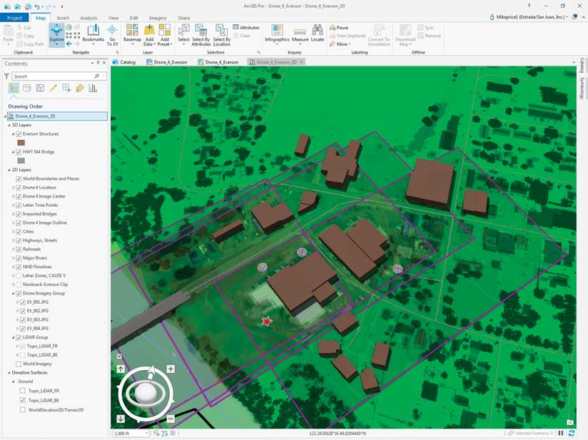
Select the Everson Structures layer and zoom to its extent. On the Appearance tab, in the Extrusion group, click the drop-down below Type and select Base Height, using the Height_M field to define the extrusion. Open Everson Structure’s Symbology pane and select a 3D Brick. From the Face Culling drop-down, choose Back.
The bridge needs shadows. In the Contents pane, right-click Drone_4_Everson_3D and select Properties. In Map Properties, select Illumination. Notice that the sun’s altitude is 90 degrees, straight down. Change this value to 45 and verify that Contrast is set to 30. Check Display shadows in 3D and click OK. Now note the shadows under the bridge and on the southeast side of buildings. Save the project again.
Studying Lahar Effects
Click the 3D Everson 1:25,000 bookmark to zoom out to the full project extent. With the Drone_4_Everson scene in 3D, some of the impacts of the lahar (volcanic mudflow) that was modeled in earlier exercises can be viewed. You will need a fast and stable Internet connection and some patience to do this portion of this tutorial.
In the Contents pane, turn off the Topo_LiDAR_FR. Expand the Lahar Zones, CAUSE V layer and turn it on. Once it appears, turn on WorldElevation3D/Terrain3D layers. Save the project. Watch the performance monitor in the lower right corner as the scene rebuilds. You will likely have to be patient to wait for WorldElevation3D/Terrain3D layer to display.
On the Appearance tab, use the transparency slider in the Effects, reduce the transparency of the Lahar Zones, CAUSE V layer to 20 percent. You can use the navigator to explore the area. North Everson and all of Nooksack are in an area designated as Zone C in the Lahar Zones, CAUSE V layer. Notice that lahar flow divides south of Everson and flows northward down Johnson Creek into the Sumas River and on to Canada.
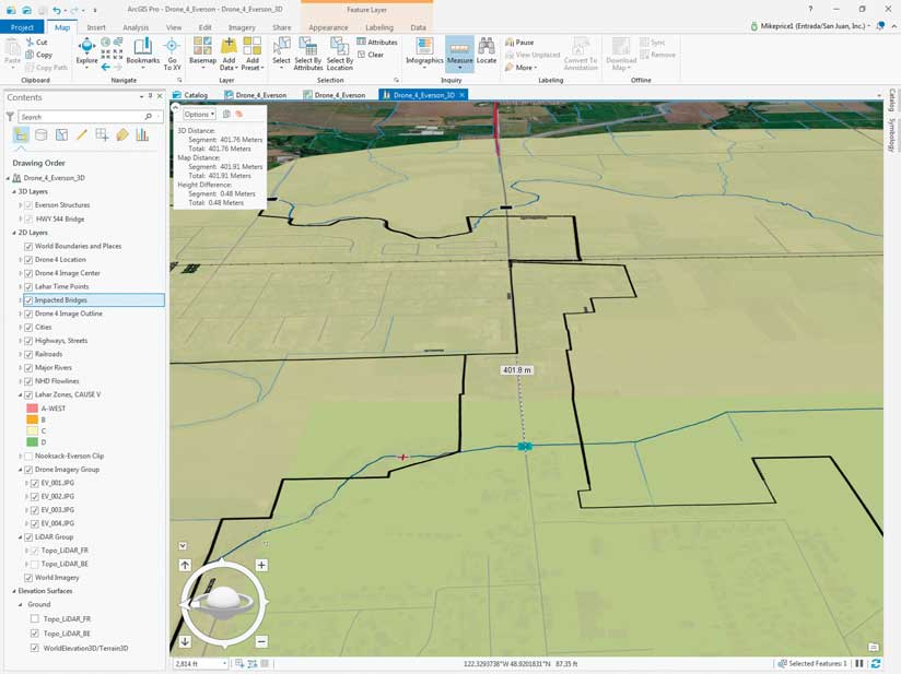
Select Impacted Bridges in the Content pane and open the attribute table. The bridges in this table are located in the modeled lahar zone and are subject to failure. To show the impact on a smaller bridge, select the Johnson Cr – E Main St bridge. Use the selected record in the table to zoom to this bridge and navigate slowly around it.
Close the attribute table. Try to view the bridge from the east and west, along the direction of traffic flow. This small bridge is a major crossing point on a Washington state highway. Nooksack floodwater may inundate a considerable length of its roadway as it is diverted toward Canada. During an actual Nooksack River flood, the inundated area can be up to 400 meters wide.
If you become disoriented when navigating through the scene, reopen the Impacted Bridges table and use the selected record to pan to the selected feature. Progress slowly, allowing the scene to fully rebuild before continuing to navigate. Save the project.
Challenge Exercises
In the most recent tutorial, “Mapping and Modeling Lidar Data with ArcGIS Pro,” hillshades were generated from bare earth and first return lidar rasters. Those rasters were also used to create contours. You can refer to the instructions in that tutorial to create those layers for this project. As you become more comfortable with ArcGIS Pro 3D capabilities, you can use your own local terrain, vector data, and images to create new scenes.
Summary
This is the final article in the CAUSE V series that started by modeling lahar travel in ArcGIS Network Analyst. Then high-resolution drone imagery was georeferenced in local coordinate space. The various transformations available in ArcGIS Pro were explored using the georeferenced lidar imagery. Next, lidar data was modeled to show detailed topography and calculate vegetation and structure heights. In this final tutorial, a 2D map of the area was converted to a 3D scene to better visualize and understand the extent and effects of the simulated mudflow.
Acknowledgments
Thanks again to Whatcom County Emergency Management and Sheriff’s Office and all CAUSE V participants. The CAUSE V data provided a great opportunity to explore ArcGIS Pro and learn about mapping and modeling natural hazards.