What You Will Need
- ArcGIS for Desktop (Basic, Standard, Advanced)
- ArcGIS Spatial Analyst extension
- Sample dataset [ZIP]
- An Internet connection
- Intermediate ArcGIS for Desktop skills
This exercise models viewsheds from Toro Peak to determine visibility for individual locations that are part of a communications network used for an earthquake early warning system in the Coachella Valley in Southern California.
A real-time earthquake warning system requires comprehensive, line-of-sight, reliable, and redundant communication. Communication systems link ground motion sensors, data processing hubs, and critical facilities in real time to detect earth movement; filter and analyze data; and quickly warn impacted facilities, even before the arrival of the most damaging waves. This article teaches how to model a viewshed and determine visibility for individual locations.
The Coachella Valley is home to some 400,000 permanent and seasonal residents. Major active faults, including segments of the San Andreas fault system, intersect the Coachella Valley. Earthquakes occur throughout the region. In 2013, the California Governor’s Office of Emergency Services (Cal-OES) began a series of stakeholder meetings to develop an implementation plan for the California Earthquake Early Warning System (CEEWS). The statewide model represents a public/private partnership. Earlier, before 2010, the Coachella Valley Regional Earthquake Warning System (CREWS) was designed and is now in implementation.
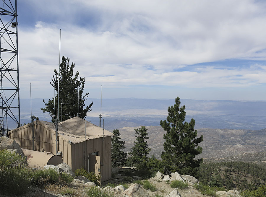
This exercise uses the ArcGIS Spatial Analyst extension to model viewsheds from Toro Peak, which looks north and east into the Coachella Valley. Its 8,717-foot-high summit is the highest peak in the Santa Barbara range.
Getting Started
To begin this exercise, download the training data [ZIP]. This dataset contains a clipped 30-meter digital elevation model (DEM) for a portion of the larger study area. The DEM is in Esri geodatabase raster format and is carefully reprojected to universal transverse Mercator (UTM) North American Datum 1983 (NAD 1983) Zone 11N.
Unzip the sample data archive on a local drive and open ArcCatalog to inspect the contents. It includes two file geodatabases, Topography.gdb and Facilities.gdb, and a collection of layer files. Topography.gdb contains the clipped and reprojected 30-meter DEM. Facilities.gdb includes three feature classes: CREWS1 and Toro_Peak1, both point layers, and Study_Area, a polygon layer. Notice that Topography contains topo_30, a file geodatabase raster dataset that does not have a hillshade. After inspecting these files, close ArcCatalog.
Preparing Data for Viewshed Modeling
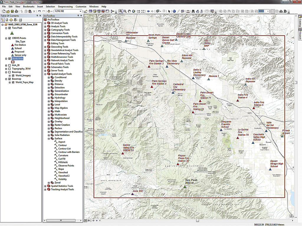
Start an ArcMap session, activate the ArcGIS Spatial Analyst extension. Navigate to \Palm_Springs. Open Toro_Peak_Viewshed1.mxd, inspect it, and repair any broken data links.
Inspect the properties of the data. Verify that all data is registered in the UTM NAD 1983 Zone 11N and that horizontal and vertical units of measure are all meters. Right-click Study Area and choose Zoom to Extent.
Look at the thematic legend for Topography, 30 M and make it the active layer. Use the Identify tool to inspect the elevation values for the 30-meter cells. These cells contain floating-point values. Before investigating the source elevation grid for these cells, let’s update the map properties.
In the Standard menu, choose File > Map Document Properties. In the Map Document Properties window, under File, verify that the path to the document is correct. Name the map Toro Peak Viewshed, and copy Topography into the Summary and Description boxes. Type your name in the Author field. Under Credit, type USGS and CREWS. This data was obtained from several agencies and modified and standardized for this exercise. Under Tags, type Coachella Valley, Palm Springs, Viewshed and separate the tags with commas. Set the default geodatabase to \Palm_Springs\GDBFiles\UTM83Z11\Topography.gdb. Check the Pathnames box and create a thumbnail. Click OK to apply these updates and save the map.
Setting Up the Geoprocessing Environment
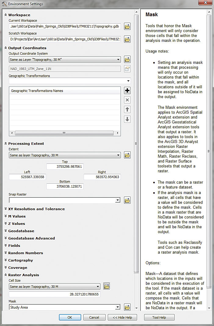
In the Standard toolbar, choose Geoprocessing > Environments. In the Environment Settings dialog box, expand Workspace and set the Current and Scratch Workspace to \Palm_Springs\GDBFiles\UTM83Z11\Topography.gdb. All the modeling results will be added to this geodatabase. Set the Output Coordinates and Processing Extent to Same as layer Topography, 30 M. Under Raster Analysis, set Cell Size to Same as layer Topography, 30 M and set Raster Analysis Mask to Study Area. Click OK and save the project.
Elevation Data Quality and Local versus Global Data
The elevation raster provided for this exercise was downloaded from The National Map. Because it has been reprojected to UTM NAD 1983 Zone 11N, the x, y, and z coordinates are all in metric units.
To replicate this exercise for another region in the United States, visit The National Map portal and download data for that area. Typically both 10- and 30-meter-resolution data is available. Although a 10-meter DEM would provide better resolution, it would be too large for this exercise, so a 30-meter DEM is used instead. Data obtained from The National Map is provided in a geographic coordinate system with NAD 1983 as the horizontal datum. Seriously consider reprojecting any data you download for another area to a standard regional metric or imperial system, using the workflow presented in “Looking Good: Properly reprojecting elevation rasters,” which ran in the fall 2013 issue of ArcUser. If x, y, and z units are identical, it is not necessary to apply vertical exaggeration.
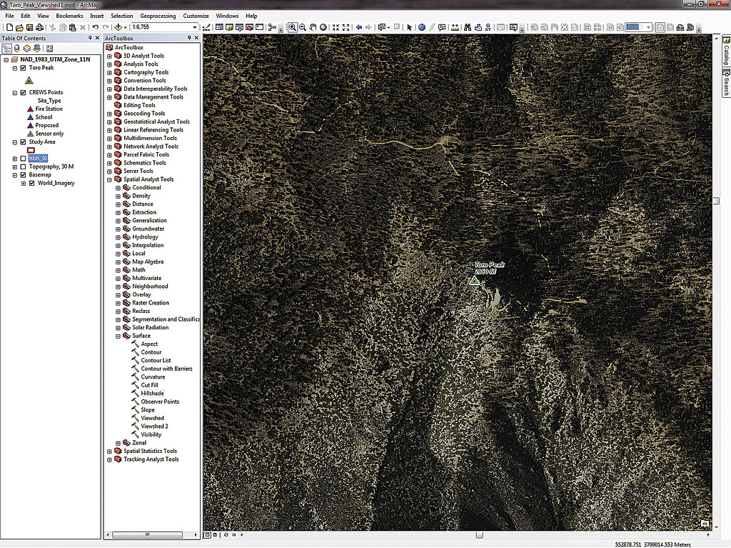
Let’s create a quick hillshade to assess the quality of this elevation data. Open ArcToolbox, expand the Spatial Analyst toolset, and locate the Surface tools. Open the Hillshade tool, set Topography, 30 M as the Input raster, and store the output raster in \Palm_Springs\GDBFiles\UTM83Z11. Name the output file hlsh_30. Accept defaults for all other parameters, and click OK. Watch as the hillshade appears.
Zoom to Toro Peak, located in the south central portion of the study area. Use the Identify tool to check elevations on and near the Toro Peak point. The highest elevation cell on the peak contains a rounded value of 2,648. This 3D point is only one meter above the raster surface. Save the map.
Using Online Basemaps
High quality basemaps are available from ArcGIS Online if you are connected to the Internet. Verify that you have an Internet connection and click the drop-down next to the Add Data icon in the Standard toolbar. Select Add Basemap and preview the available maps. Select Imagery, and wait patiently as recent high-resolution imagery loads as a basemap layer. All basemap layers load at the bottom of the table of contents (TOC).
Zoom in until the scale is approximately 1:6,000, and study the transmitter point. The antenna is on the northwest corner of the structure that contains the communication equipment. The tower, located at the top of the mountain, faces north toward the Coachella Valley.
Right-click on the Study Area layer and choose Zoom to layer. Uncheck but don’t remove the World_Imagery basemap, and turn off the hlsh_30 and Topography, 30 M layers. Reopen the Basemap gallery and select Topographic. World_Topo_Basemap will be used for the rest of the exercise. After the new basemap loads, save the project.

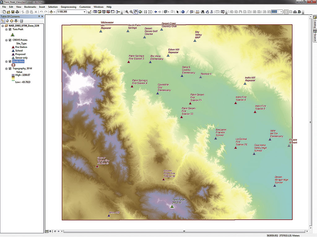
Explore the CREWS points. Study the relationship of CREWS sensor and facility points relative to topography, streets, and political boundaries. Most CREWS points lie within one of the Coachella Valley municipalities: Palm Springs, Cathedral City, Rancho Mirage, Palm Desert, and Indio. CREWS points include schools, fire stations, and raw sensor locations.
Several sensors, including one proposed location, are at high elevations. When an earthquake occurs, sensors need to quickly collect and stream seismic data to one or more communication facilities, where it will be processed and alerts generated. Alerts are sent to essential and critical facilities either by wireless communication or via the Internet.
Since instantaneous communications are essential, CREWS points should be in the line-of-sight viewshed of a major communications hub. Toro Peak’s location and elevation suggest that it might be an excellent location for such a hub, as it could “see” most or all CREWS points. Let’s model the Toro Peak viewshed with the Viewshed and Viewshed 2 tools in the Spatial Analyst toolbox.
The Original Viewshed Tool
For many years, the Spatial Analyst extension provided a Viewshed tool that can be used to create a simple viewshed. In ArcToolbox, expand Spatial Analyst Tools and choose Surface Tools > Viewshed. Set the Input raster to Topography, 30 M. Set Input points or polylines to Toro Peak. Name the Output raster VS01_01_00. This output naming convention references the original Viewshed tool (VS01), the observation elevation (i.e., antenna height) to 01, which is one meter above the elevation raster, and the surface height to 00, which is not readily available in Viewshed).
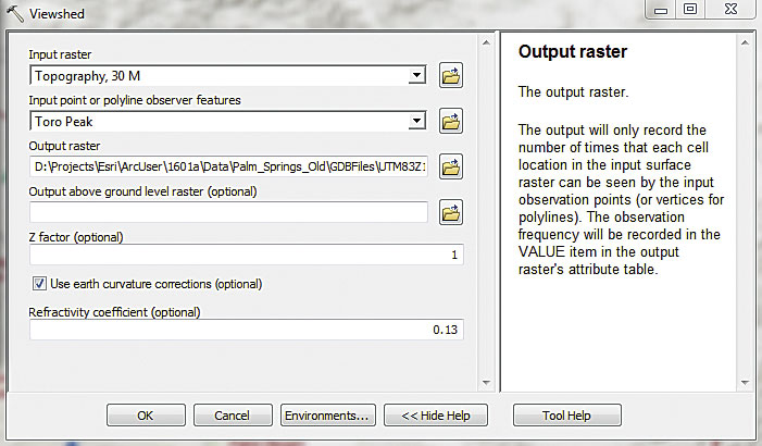
Since all units are meters, leave the z factor as 1. Check the Use earth curvature corrections box and click OK.
When the Viewshed tool loads, ArcGIS assigns standard pink and green colors to the cells. A nonvisible cell has a value of 0 and is pink, and a visible cell has a value of 1 and is light green. In the TOC, place VS01_01_00 below hlsh_30.
To standardize the legend and hide nonvisible cells, use symbology from the Viewshed_1 layer file. In the TOC, right-click VS01_01_00, open Properties, and select Symbology. Verify that Show is set to Unique Values and open Import. Browse to \Palm_Springs\GDBFiles\UTM83Z11 and select Viewshed 1.lyr. Click OK to apply symbology. The visible cells are now Leaf Green. Next, click Display and set transparency to 60. Transparency allows the underlying basemap to display below the Viewshed. (To see the visible cells even more easily, turn off the basemap layer.) Save the project. Zoom in to southern Palm Springs and study the viewshed.
Palm Springs Fire Station 3 is just inside the Toro Peak viewshed, but Station 4 is not. Pinyon Pines Station 30 and several schools are also outside the modeled viewshed. Now, let’s use the Viewshed 2 tool to raise antennae and see if visibility improves. Turn off VS01_01_00 and save the map.

The New Viewshed 2 Tool
In 2015, the Viewshed 2 tool was added. It includes several significant improvements over the previous Viewshed tool. Viewshed 2 is available with a Spatial Analyst or 3D Analyst license. It determines raster surface locations that are visible to a set of observer features using geodesic methods. Each cell’s visibility is determined by a line-of-sight test between the target and each observer. If an observer can see the target at the cell center, the cell is considered visible. Nonvisible cells are assigned NoData. When modeling visibility, the tool always considers the curvature of the earth and does not have a z-factor parameter.
The tool exposes many new user-defined variables, including observer and viewed object heights above an elevation raster, maximum and minimum modeling radii, and viewshed azimuth constraints. If a graphics processing unit (GPU) is available on your computer, it will be used to enhance the performance of the Viewshed 2 tool.
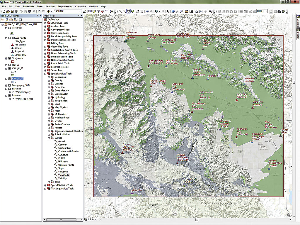
Zoom to the Study Area layer, return to Surface tools, and open Viewshed 2. Set the Input raster to Topography, 30 M and name the Output raster VS02_21_05. By raising the 5-meter Toro Peak antenna to 21 meters, it will be above all CREWS points. Expand and review Viewshed parameters. Accept all defaults and expand and study Observer parameters. Set Surface offset (the CREWS points) to 5 meters and set Observer offset to 20 meters to place (virtually) a 20-meter antenna on Toro Peak and 5-meter antennae on all CREWS points. Save the project and click OK to model Viewshed 2. These are complex calculations that may take a while to process.
When VS02_21_05 loads, move it immediately below SV01_01_00. Open Properties, click Symbology, and set the classification to Unique values (this is very important). If asked to create an attribute table, click Yes. While still on the Symbology tab, use Viewshed 2.lyr to apply Dark Navy symbology. Set transparency to 60 percent, click OK, and save again.
Inspect the relationship of VS01 and VS02, especially in southern areas. Notice that Fire Stations 30 and 53 are now visible, as is the proposed sensor Anza SW at the Benjamin Franklin School, which is very close to visible, but several other schools and Fire Station 3 are still not visible. Unfortunately, the hills immediately south of the Coachella Valley floor are too high to expose these points. Save the project.
Converting a Viewshed Raster to a Polygon Feature Class
For some mapping and analysis, polygon representations of Viewshed perimeters are very useful. Let’s convert VS01_21_05 to a polygon feature class. In ArcToolbox, locate the Conversion toolset, choose From Raster > Raster to Polygon. Set VS02_21_05 as the input raster, set the field as Value, and name the output raster VS02_21_05_p (p for polygon) and store it in Topography.gdb. Click OK to continue and place the filled polygon above hlsh_30.
Rename the viewshed polygon Viewshed 21, 5. The numbers represent the Toro Peak and CREWS antenna heights. Instead of applying transparency to this viewshed polygon, apply a No Color or Hollow fill color and a 2 point ultra blue outline. Save again.
Let’s select all CREWS points that lie inside the enhanced visibility area. In the Standard menu, choose Selection > Select by Location. Accept the default Select features from method and specify CREWS Points as the Target layer. Set Viewshed 21, 5 as the source layer and specify the Intersect the source layer feature method. Do not check the box next to Apply a search distance. Click OK to select visible CREWS points. Open the CREWS Points attribute table and inspect selected records. With a 21-meter antenna on Toro Peak and 5-meter antennae on all CREWS sites, you could have 21 selected site records out of 26 total sites. Switch the selection and study the five nonvisible sites. The project is finished, so save it.
Seeing Hidden Stations
The Visibility 2 tool showed that 21 of 26 CREWS points with 5-meter antennae are visible from a 21-meter high antenna on Toro Peak. Review all nonvisible points to consider other methods to efficiently “see” them.
Notice the three repeater sites in the north. Perhaps they can see the five hidden sites. It might be possible to raise the Toro Peak antenna to see one or more sites or install higher antennae on certain CREWS locations. If you experiment with antenna height, you will likely find that topography immediately south of the Coachella Valley floor is too rugged to overcome with higher antennae. Repeaters or land links could be the answer, although the time interval might be too great to provide the desired warning window.
Get ready for earthquakes by developing and practicing a readiness plan. Get more earthquake safety information.
Acknowledgments
This exercise includes elevation raster data downloaded from The National Map portal and facility and sensor point data from the Coachella Valley Regional Earthquake Warning System. It also used ArcGIS Online basemaps provided by Esri. Special thanks to Blake G. Goetz, regional director/IHUB director for Southern California Earthquake Warning System. Special thanks also to Seismic Warning Systems, Inc., for invaluable guidance on program scope and modeling needs.
See also “Partnerships Provide Earthquake Warning in California” and “Understanding Earthquake Early Warning Systems.”