GIS analysts use point data to model complex trend surfaces. Field data is often collected at irregularly distributed locations, and attributes are sometimes difficult to consistently quantify. Also, barriers such as geologic faults, watershed boundaries, and urban canyons may influence local interpolation.
The tools in the ArcGIS Geostatistical Analyst extension allow GIS users to analyze spatial trends within complex point datasets and model predictive surfaces that best represent data trends. Empirical Bayesian Kriging (EBK) provides powerful data analysis tools, including variography of data in space. Kernel Smoothing interpolates irregular surfaces and predicts standard error throughout the model. By including polyline or polygon barriers, Kernel Smoothing With Barriers can accurately model point data within discrete subgroups.
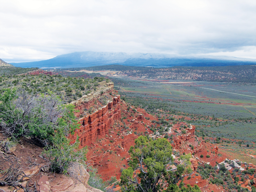
This tutorial teaches how to use the ArcGIS Geostatistical Analyst and Spatial Analyst extensions to explore and evaluate data using data that describes an oil field in Lisbon, Utah, and synthetic data created just for this exercise. Read the accompanying article below, “About Lisbon Valley,” to learn more about this geologicly interesting area.
The exercise begins by using the EBK tool in Geostatistical Analyst to explore geologic borehole data. Then Spatial Analyst is used to interpolate a geologic/structural surface (formation top) using the Spline With Barriers tool. Precinct elevation values and a surface for the same geologic/structural surface will be created using Kernel Smoothing With Barriers tool in Geostatistical Analyst. Finally, a Prediction Standard Error (PSE) for the Kernel Smoothing predictive surface will be created. The resultant Kernel Smoothing surface is compared to the surface created with Spatial Analyst using Spline With Barriers. For an overview of the Geostatistical Analyst tools used in this tutorial, see “A Little More about Two Geostatistical Methods” in this issue.
Getting Started
First, download the sample dataset [ZIP] and unzip the archive on a local computer.
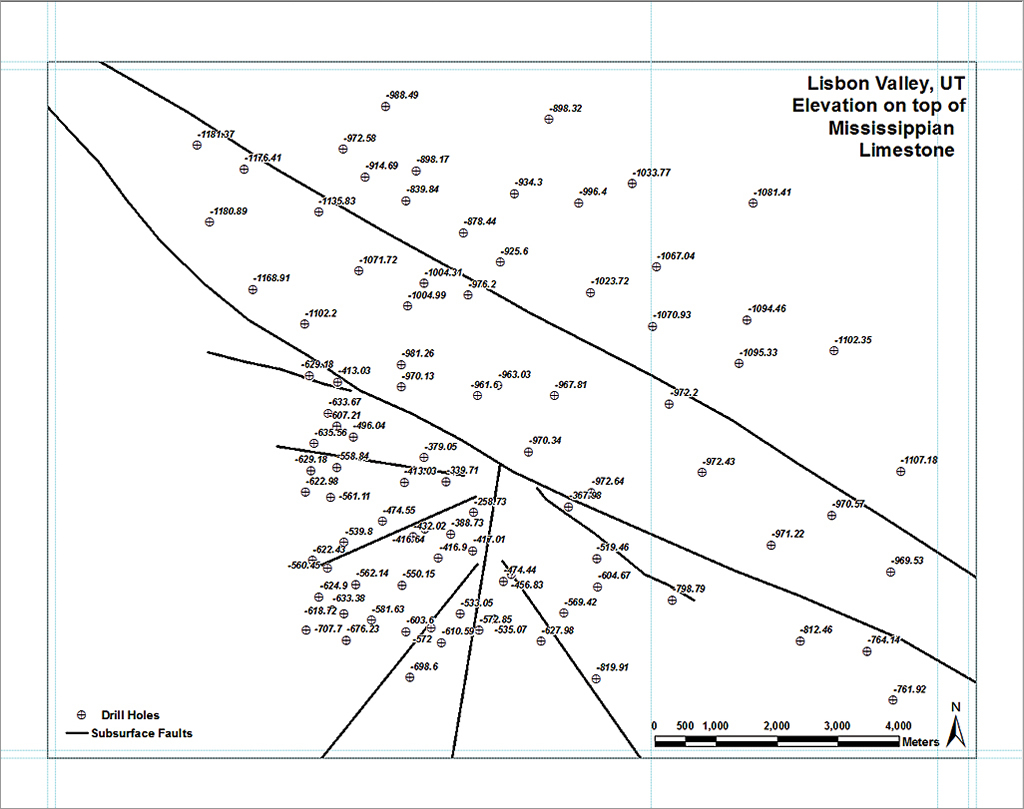
- Start ArcMap, navigate to \Lisbon_UT, and open Lisbon_Valley_UT.mxd. This map document opens in layout view and shows the locations of drill holes and subsurface faults. It includes data from three file geodatabase feature class layers—Drill Holes, Subsurface Faults, and Clipping Grid.
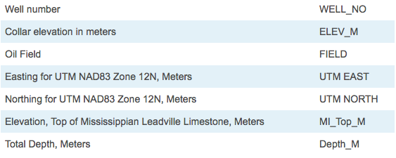
- In the table of contents (TOC), open the attribute table for Drill Holes and explore its fields. This table includes 91 drill holes, both real and synthetic. Study the data in the MI_Top_M field. It will be analyzed and modeled throughout this exercise. Close the table.
- Switch to data view and choose Bookmark > Lisbon 1:50,000.
- Update the map document by specifying a default geodatabase. In the ArcMap Standard menu, choose File > Map Document Properties. Set the Default Geodatabase to \Lisbon_UT\Geodatabase\UTM83Z12\Lisbon_Geology.gdb.
- Check Store relative paths and click the button to create a thumbnail. Click OK.
- Select Customize > Extensions and verify that the Geostatistical Analyst and Spatial Analyst extensions are installed and checked. Open the Geostatistical Analyst and Spatial Analyst toolbars by clicking an open area on any toolbar and selecting Geostatistical Analyst and Spatial Analyst from the available toolbars.
- Dock the Geostatistical Analyst toolbar in the upper left of the interface and click the drop-down. The Geostatistical Wizard will be used to access the tools used in this exercise. The Geostatistical Wizard can also be accessed by clicking a single button on the toolbar. The drop-down also contains Explore Data, Create Subsets, Help, and Tutorial choices.
Setting Environments
An essential—and occasionally overlooked—step is defining geoprocessing environments for this map. When creating an ArcMap document that includes geoprocessing, it is very helpful to include one or more reference rasters to define and guide processes. Clipping Grid is the reference grid for this exercise. Momentarily display it to see the extent of the model. Note the extent includes all drill holes. With 10-meter raster cells, it will have excellent data resolution.
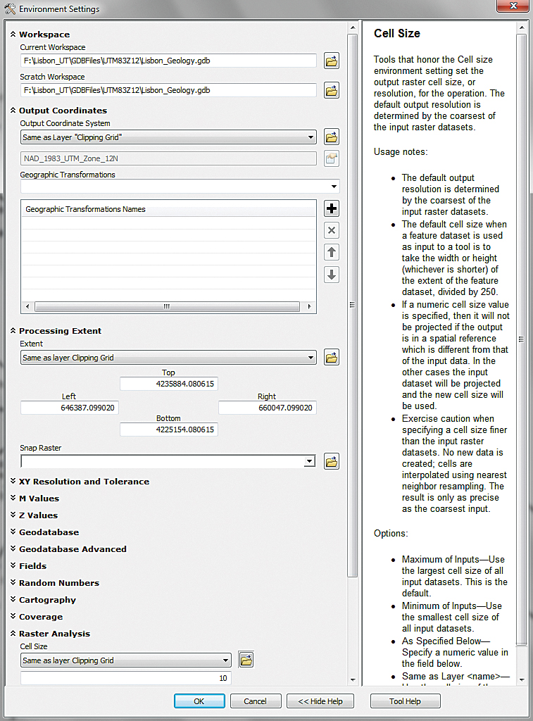
- In the Standard menu, choose Geoprocessing > Environments and expand Workspace. Verify that the Current and Scratch Workspaces are both set to \Lisbon_UT\Geodatabase\UTM83Z12\ Lisbon_Geology.gdb. This was the same geodatabase specified in the Map Document properties.
- Expand Output Coordinates and set Output coordinate system to Clipping Grid. When performing geostatistical analyses, it is highly desirable to apply a nongeographic coordinate system so this exercise will use a projected coordinate system, universal transverse Mercator.
- Expand Processing Extent and set the extent to Same as layer “Clipping Grid”.
- Expand Raster Analysis and set the cell size to Same as layer “Clipping Grid”.
- Click OK to apply these updates and save the file.
Exploring Data with EBK
In the Geostatistical Analyst toolbar, open the Geostatistical Wizard. Under Methods, there are three separate groups: Deterministic methods, Geostatistical methods, and Interpolation with barriers. Expand the headings for each method to inspect the tools.
- Choose Empirical Bayesian Kriging (EBK), located under Geostatistical Methods. It opens to the first pane in the wizard, the Input Data pane. Using drop-downs, set Source Data to Drill Holes and specify MI_Top_M as the Data Field. Click Next to continue.
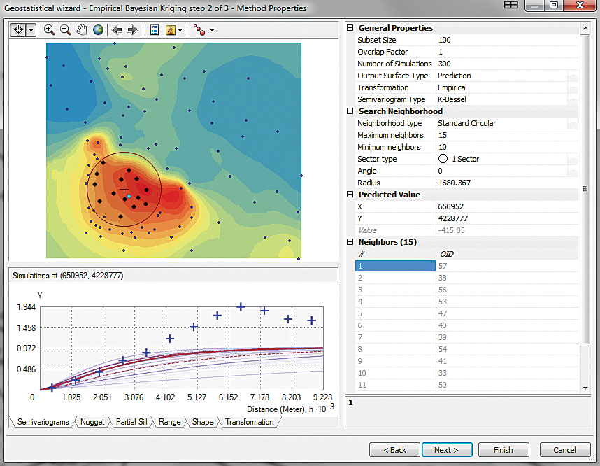
- In the Step 2 pane of the wizard, update some of the analysis properties under General Properties in this order:
- Increase Number of Simulations to 300.
- Change Output Surface Type to Prediction.
- Set Transformation to Empirical.
- Specify a K-Bessel Semivariogram Type.
- Do not change Search Radius for the first pass through this data or your results will differ from the examples in this exercise.
- Expand the Neighbors area and use explore the model by selecting points within the search radius. With each mouse click, the X, Y, and Value (MI_Top_M) coordinates are updated. These are the 10 points used to predict the value at the circle’s center. Inspect the EBK surface displayed in the wizard and notice that there appears to be three separate point groups: a major group in the southwest, a smaller northeast group, and a central band trending from southeast to northwest. Although faults are not shown on this map, they are important. EBK does not include polyline or polygon barriers, so this exercise will test two alternate interpolation methods.
- Still in the Step 2 pane, explore the Nugget, Partial Sill, and other tabs. Click Next to continue.
- The Step 3 pane displays the Cross Validation matrix for the EBK analysis. Points can be sorted using Error. Outlier points can also be selected. Select points at both ends of the sorted data to highlight outliers. Look at the other Cross Validation tabs for Error, Standardized Error, and Normal QQPlot. Click Finish.
- In the Method Report window, click the Save button and save the parameters as an XML file. Save the EBK parameters in a new folder named \Lisbon_UT\Results, accept the default name, and click OK.
- The EBK prediction surface layer will be generated and appear in the map document. In the TOC, move it below Subsurface Faults and inspect the relationships between the prediction and the faults. Areas of similar predicted values extend slightly across faults. There are at least three distinct regions that could be separated by major northwest trending faults.
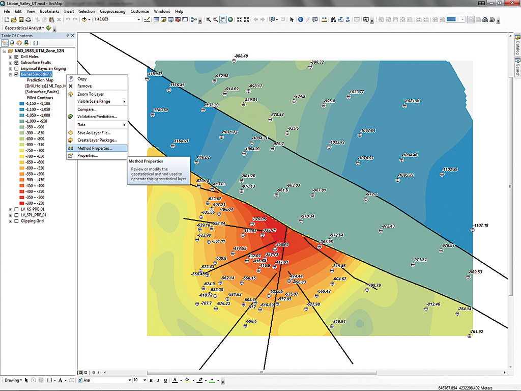
- Right-click the Empirical Bayesian Kriging layer and select Properties. Click the Symbology tab. Hillshade, Contours, Grid, and Filled Contours can be displayed. Check Contours and Filled Contours. To see the displayed Contours, change their symbology to a single dark line. Check Presentation quality and Refine on zoom. Click OK.
- Save the map document.

Using Spline with Barriers
EBK predictions use points on both sides of a fault. Let’s try an interpolation/prediction method available with the Spatial Analyst extension that respect fault barriers.
- In the TOC, collapse the Empirical Bayesian Kriging layer and turn it off. Choose Bookmark > Lisbon 1:50,000 to adjust the displayed extent.
- Open the Search box and locate Spline With Barriers (Spatial Analyst).
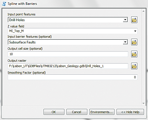
- In the tool, select Drill Holes as the Input point features and select MI_Top_M as the Z value. Choose Load Subsurface Faults as the Input barrier features, leave Output cell size as 10, and Smoothing as 0. Save the output raster in \Lisbon_Geology.gdb as LV_SPL_PRE_01. Click OK.
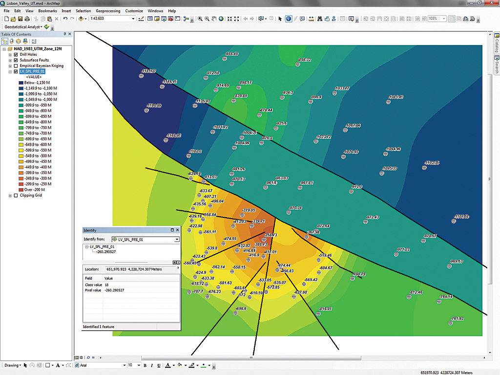
- After the spline raster appears, move it down in the TOC below the EBK layer. Right-click LV_SPL_PRE_01, select Properties, and open the Symbology tab. Change Show: to Classified and use the symbology import browser to load SPL Prediction, Meters.lyr, located in \Lisbon_UT_Geodatabase\UTN83Z12.
Inspect the splined raster and notice the abrupt changes across faults. Use the Identify tool to explore the raster. Although this output looks acceptable, there is no way to measure error throughout the model. Let’s return to Geostatistical Analyst and try Kernel Smoothing. Close ArcToolbox, turn off LV_SPL_PRE_01, use the Lisbon 1:50,000 bookmark to adjust the extent, close Search, and save the project.

Using Kernel Smoothing With Barriers
- Return to the Geostatistical Wizard and, under Interpolation With Barriers, select Kernel Smoothing.
- In the Kernel Smoothing Wizard, set Drill Holes as the Source Dataset and MI_Top_M as the Data Field. Set Subsurface Faults as the Barrier Features Source Dataset and click Next.
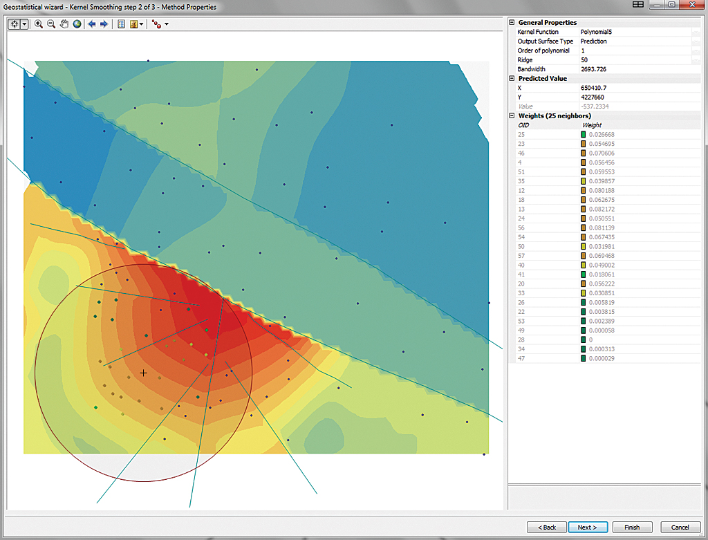
- After the Kernel Smoothing prediction surface appears, accept all defaults and zoom in on the active prediction surface. Notice that fault barriers now appear in the wizard and that the model appears to respect them.
- Move the selection circle through the model by clicking the crosshair on various points and inspect predicted values. The default search radius or Bandwidth is now nearly 2,700 meters. Click Next.
- Inspect the Cross Validation charts on the Predicted and Normal QQPlot tabs. The points fall much closer to the Regression line. Click Finish.
- Click the Save button and save the model summary as an XML file called Kernel Smoothing in the Results folder in the Lisbon_Geology.gdb. Click OK.
Enhancing Kernel Smoothing Model
- In the TOC, move the Kernel Smoothing layer just above Clipping Grid, right-click it, and select Properties.
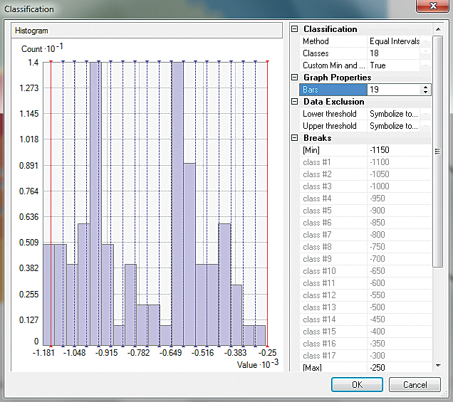
- Open the Symbology tab, check Filled Contours, and select Classify. Under Classification, change Method to Equal Intervals, set Classes to 18, and set Customize Min and Max to True (this last step is very important).
- In Graph Properties, set Bars to 19. At the top of Breaks, set a Min break at -1150. Move to the bottom and set a Max value of -250 (below sea level). Click OK to reclassify. The classified intervals are now 50 meters wide.
- Check the Presentation quality and Refine on zoom options so more raster detail will be displayed and the jagged edges along faults will be minimized. Click OK.
- Export the Kernel Smoothing Prediction surface as a geodatabase raster. In the TOC, right-click on the Kernel Smoothing layer, select Data > Export to Raster. Save the prediction raster in Lisbon_Geology.gdb, naming it LV_KS_PRE_01. Be patient as it loads. Move it just above Clipping Grid, collapse its legend, and turn it off.
Modeling Predicted Standard Error (PSE)
Because Kernel Smoothing is a tool available in Geostatistical Analyst, a predictive elevation surface and an estimate of standard error across the surface can be created. First, the error threshold throughout the model will be estimated in meters. Error will likely be lowest within clustered points and may be highest on the edge of drilling and near barrier faults.
- Save the file and return to the TOC. Right-click Kernel Smoothing and open Method Properties.
- In Wizard Step 1, change Output Surface Type to Prediction Standard Error. A new raster will appear. This raster displays the predicted margin of error for the Mississippian limestone top throughout the model. Error in meters is smallest in the drilling clustered in the southwest portion and greatest along outer margins and along faults. Within the drilling cluster, predicted error is highest near barrier junctions involving three faults, especially within narrow fault blocks.
- Click Next to display the Cross Validation charts. Reinspect these charts, especially those on the Error and Standardized Error tabs.
- The next step will plot these points on the map. In the lower right side of the wizard pane, scroll down to Export Result Table and click the plus sign next to it. Export the points to Lisbon_Geology.gdb and name the file LV_KS_CrossValidationResult. Click Finish. Verify that this new layer loads at the top of the TOC. Do not save the Method Report.
- Right-click Kernel Smoothing, select Properties, and open Symbology. Change the Classification Method back to Geometric Intervals, and set Classes to 20. Leave all other default values, click OK, check both Presentation quality and Refine on zoom, and click OK again.
- Turn on LV_KS_CrossValidationResult and open its table. Select Error and sort the table in ascending order. Use sorting and selection to identify points with the highest positive and negative errors. You should find that they are often near the model edge or in areas of tight barrier polyline convergence, as expected.
- Export the Kernel Smoothing raster and save it in Lisbon_Geology.gdb as LV_KS_PSE_01. Update the legend using KS Prediction Standard Error.lyr. Finally, use Layer file KS Prediction, Meters.lyr to update the legend for LV_KS_PRE_01 and save the file.
Conclusion
This exercise showed how to model the elevation of the top of the Mississippian limestone in Lisbon Valley, Utah, using only formation top elevations and fault barriers to generate a reliable predictive elevation surface. Predicted standard error across the surface was also created. These surfaces were exported as rasters.
Acknowledgments
Thanks to Konstantin Krivoruchko and the Esri Geostatistical Analyst team for their help in developing the exercise workflow. Thanks, also, to the many geoscientists who have visited Lisbon Valley and developed an extensive and enduring understanding of the area.