What you will need
- ArcGIS Pro 2.1 license
- ArcGIS Online for Organizations account
- Sample dataset downloaded from the ArcUser website [ZIP]
- An unzipping utility
This tutorial introduces georeferencing techniques available in ArcGIS Pro using imagery collected by drones during a multi-day training exercise testing response and recovery capabilities of US and Canadian emergency agencies. The training exercise was held across the westernmost portion of the US-Canada border.
During the week of November 13, 2017, public safety agencies in the United States and Canada, supported by other governmental and industry participants, conducted the fifth Canada-United States Enhanced Resiliency Experiment (CAUSE V) exercise. The scenario for this exercise, which was also the basis for a tutorial in the summer 2017 issue of ArcUser, “Modeling Volcanic Mudflow Travel Time with ArcGIS Pro and ArcGIS Network Analyst,” included a hypothetical crater collapse on Mount Baker, a dormant composite volcano with accompanying seismic activity that would result in volcanic mud and debris flows (lahars), riverine flooding, landslides, and other natural phenomena. To learn more about CAUSEV and Mount Baker, read “Testing Cross-Border Disaster Response Coordination” and “Mount Baker (Briefly)” in the fall 2017 issue of ArcUser.
An Overview of Georeferencing
Raster data can be obtained from many sources including satellite sensors, aerial cameras, scanned maps, and drawings. Many current capture technologies can extract coordinate information, embedding it in or providing it with imagery. Older scanned aerial photos and maps must be georeferenced. Although they might display in local or regional coordinate systems, they must be repositioned to fit a flat object into a spherical coordinate system.
Sometimes, it is necessary to locally fine-tune georeferencing. By georeferencing a raster, it can be viewed, digitized, and analyzed with other data in the coordinate system that was applied. To georeference a raster requires that you
Add the target raster to a projected map that includes appropriate reference data.
Create control points and connect them with the corresponding reference point locations on the raster.
Review control points and edit them or add additional points as necessary.
Assign an appropriate transformation that is based on the number and distribution of control points.
Save the georeferencing information with the raster or export the georeferenced raster as a new raster.
About the Imagery Used
To support data collection and analysis during the CAUSE V exercise, drones and robots were deployed at multiple locations to collect data via remote sensors. Field data was transmitted back to the Whatcom County Emergency Operations Center (EOC) in Bellingham, Washington, in real time, using land-based broadband and satellite technologies.
Imagery was captured by a DJI Phantom4 drone provided by TacSat Networks Corporation of Santa Clara, California. TacSat Networks specializes in the integration, delivery, and sale of deployable secure wireless communications for public disaster emergency response agencies and the private sector in the United States and overseas.
The drone sent streaming video and still images back to the EOC over its ViaSat Pro2 Ka-band satellite network. Three separate locations in Washington were supported: Newhalem on November 15 and Deming and Everson on November 16. The drone and deployable satellite communications were quickly remobilized between sites, and communications were established throughout both days.
Four high-resolution still nadir (down-looking) images taken from the Everson location were delivered as JPEG files without orthorectification. These images included a return flight path over the Washington Highway 544 bridge and the southwestern portion of the town of Everson, just north of the Nooksack River.
In “Modeling Volcanic Mudflow Travel Time with ArcGIS Pro and ArcGIS Network Analyst,” it was estimated that the path of the lahar (volcanic mudflow from Mount Baker) down the Middle Fork Nooksack would reach the Everson bridge in approximately 120 minutes, hitting the bridge and possibly flowing into Everson.
Drone imagery enabled incident managers at the EOC to view areas that would experience lahar and riverine flooding for several miles up and down the Nooksack River. This tutorial uses two of several raster images captured by drones and places them on a map using the universal transverse Mercator (UTM NAD 1983) Zone 10N projection.
Getting Started
Begin by downloading the sample dataset for this exercise from the ArcUser website (esri.com/esri-news/arcuser) to a local drive. Cause_V_Drone_4.zip contains several file geodatabases, four training JPEG images, and an MXD file that will be imported into ArcGIS Pro. Unzip the sample dataset archive to a local drive.
Start ArcGIS Pro and choose new Blank project. When prompted, create a new project, name it Drone_4_Everson, and store it in Cause_V_Drone_4. Make sure you store your project in the Cause_V_Drone_4 folder. Once the ArcGIS Pro map opens, select the Insert tab and click Import Map. Navigate to Cause_V_Drone_4, select Drone_4_Everson.mxd, and click OK.
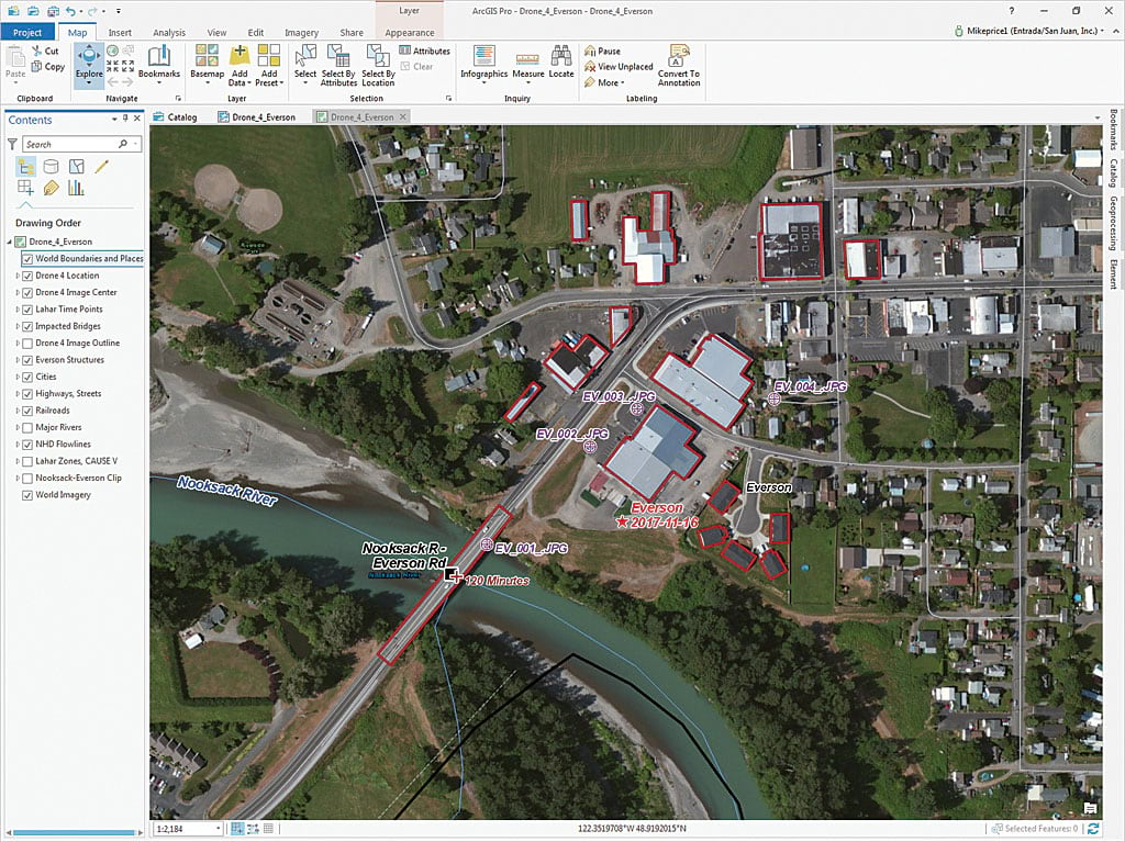
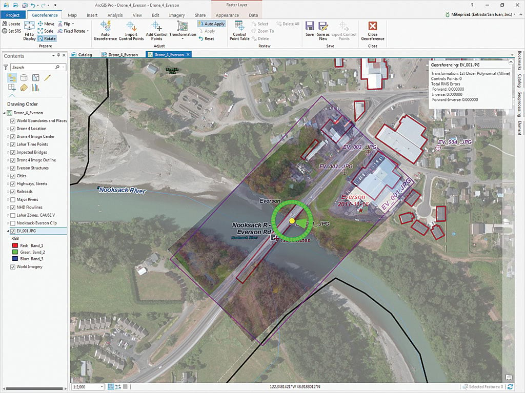
Inspect the map just imported. The map’s current extent shows the Nooksack River flowing west in the southwest corner of Everson and contains a local transportation layer. The layout’s map scale is 1:2,500.
Open the Catalog pane, expand Maps, right-click Drone_4_Everson, and choose Open. The imported map opens on a new tab as an ArcGIS Pro map with the same name. The imported map is linked to the ArcGIS Pro map. The map should be in map view, which will be used to georeference images.
Click the basemap drop-down and select Image with Labels. The high-resolution basemap shows the southwest corner of Everson, the Nooksack River, and the Highway 544 bridge. Turn on the Drone4 Location, Drone 4 Image Center, Lahar Time Points, Impacted Bridges, and Everson Structures layers. Turn off Major Rivers. Leave the layers that were already on alone. Inspect the map. Save the project.
Using Reference Image Foot-prints to Create Control Points
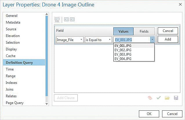
The Drone 4 Image Outline layer contains outlines for all four image files. Using a definition query will let you limit the number of image outlines displayed to just one.
In the Contents pane, turn on and right-click the Drone 4 Image Outline layer. Open Properties, select Definition Query, and click Add Clause. In the query builder, create the expression Image_File is Equal to EV_001.jpg. Click OK to apply. Right-click the Drone4 Image Outline layer and choose Zoom to layer.
Click the Imagery tab and locate the Georeferencing tool. Click the small Alignment button on the lower-right corner. The Georeferencing Options window allows you to customize the tools. Accept all defaults and close the window. Save the project again.
Add and Transform EV_001.JPG
Click the Map tab and click Add Data > Data to add data to the map. Navigate to \CAUSE_V_Drone_4\Imagery\Everson Images and select EV_001.JPG. Verify that the image loaded in the Contents pane immediately above the World Imagery basemap. Inspect several Structure Footprints, including the bridge deck and several buildings, which are outlined in red. The Nooksack R-Everson Road bridge is on the list of essential and critical facilities. The drone was used to carefully inspect the bridge and photograph the floating material trapped on its northern abutment.
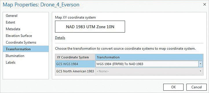
In the Contents pane, select EV_001.JPG, click the Imagery tab, and click Georeference. Notice the Georeferencing window in the upper-right corner. On the far left of the Georeference ribbon, click the Set SRS (for spatial reference system) button. Confirm that the Map XY coordinate system is NAD 1983 UTM Zone 10N.
Click Transformation and set the transformation from GCS WGS 1984 to WGS 1984 (ITRF00) TO NAD 1983. Click OK to apply and save again.
Get Ready to Georeference
In the map, right-click the Drone 4 Image Outline layer and choose Zoom to layer. Write down the scale visible in the lower-left corner.
Calculate two-thirds of that scale value (for example, if the scale at Zoom to layer is 3,000, then change the scale to 2,000).
On the Georeference ribbon, click Fit to Display.
To deemphasize the underlying raster, select World Imagery in the Contents pane, click the Appearance tab, and set Layer Transparency in the Effects group to 40percent.
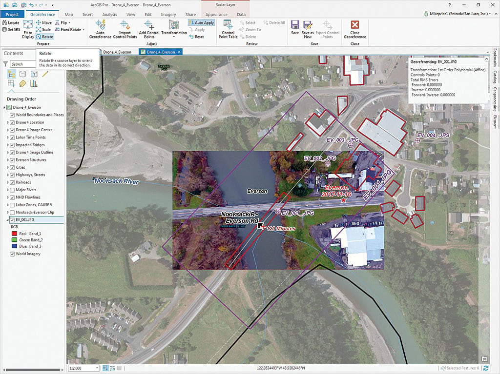
ArcGIS Pro includes a powerful image rotation tool in the Georeference toolset. In the Contents pane, select EV_001 and, with the Georeference ribbon active, select Rotate (not Fixed Rotate). Move your cursor over the center of EV_001 and study the live rotation graphic. Hold the left mouse button down on the green circle and rotate the raster until it closely fits its image outline.
This image requires a counterclockwise rotation of approximately 30 degrees. Don’t worry about being too precise because four control points will be set—one on each footprint corner. Save the project to preserve these changes. If your raster image behaves badly, simply reload it and start over.
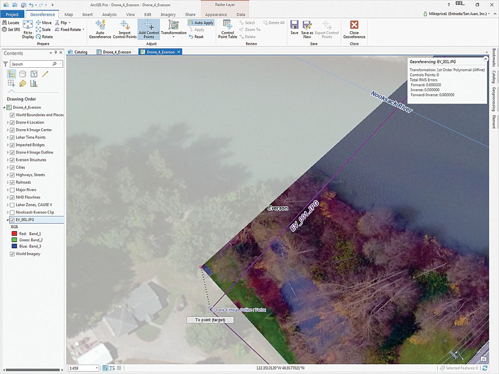
Zoom to the southwestern corner of the rotated image and its outline and inspect the relationship between the outline and image.
Before creating a control point to connect the raster corner to the same corner in the reference Image Outline, click the Edit tab, open the Snapping tool on the Editing ribbon, and confirm that only Vertex Snapping is available.
Creating Easy Control Points for EV_001.JPG
Return to the Georeference ribbon, verify that EV_001.JPG is selected, and click the Add Control Points tool located in the Adjust group. Locate and left-click the southwest corner of the image and confirm that From point (source) is active. Move your cursor to the southwest reference polygon corner, allow it to snap, and click again to create a To point (target).
Move diagonally to the raster’s northeast corner and create a second control point. Move to the northwest corner and create a third control point, then create the fourth and final control point at the southeast corner.
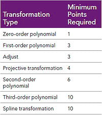
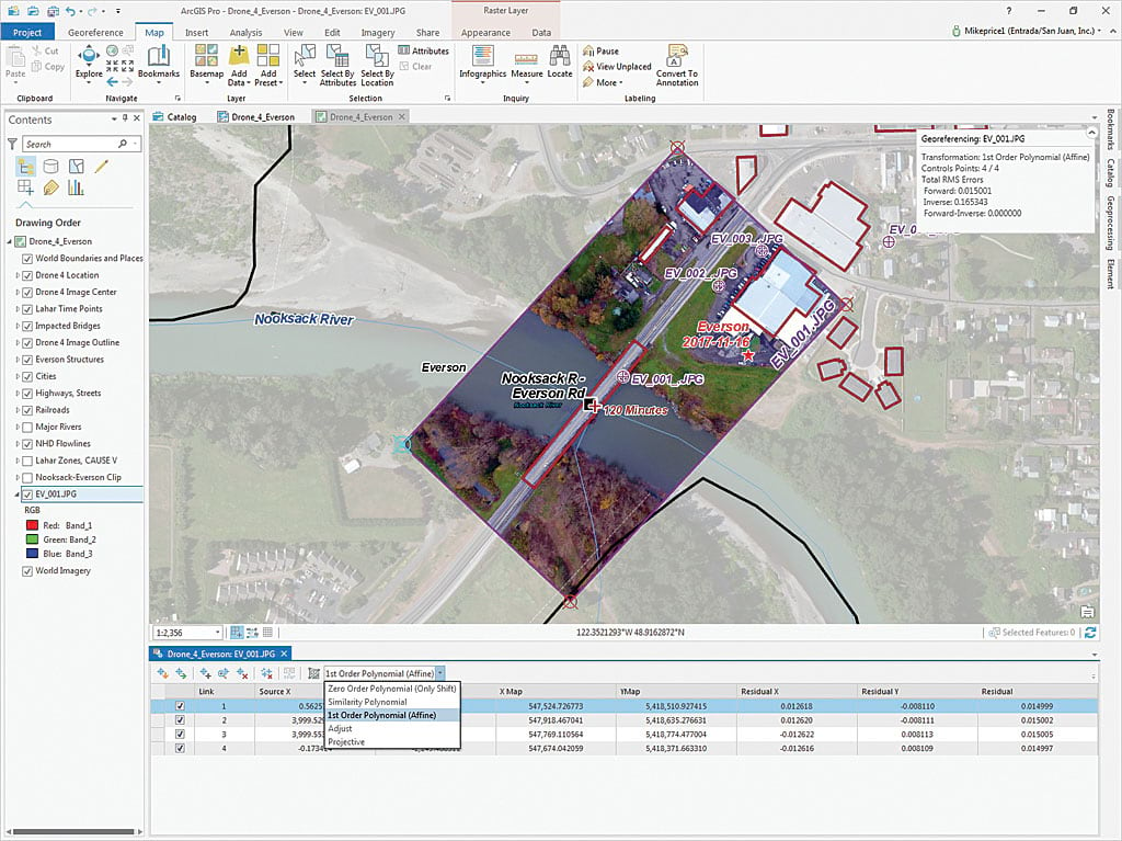
Open the Control Point Table, located in the Georeference Review group. In the Control Point Table, inspect the transformations available from the Transforms drop-down and review Table 1, which shows the number of points required for different transformation types. In the Control Point Table, select individual records. Because only four control points were created, the number of transformations available is limited.
Now, it’s time to decide how to preserve the updated image. There are two options: update the georeferencing for the current image or save the image as a new transformed image. To ensure the registration can be fine-tuned later, temporarily save the control information by locating the Georeference Save group and clicking Save. Click the Close Georeferencing tool located on the right end of the Georeference ribbon.
More carefully inspect the georeferenced image by selecting EV_001, opening the Appearance ribbon, and choosing the Swipe tool. Use the Swipe tool to reveal the underlying World Imagery and compare structures in EV_001 with the same structures on the basemap image. Also compare structures shown in EV_001 with the outlines in the Everson Structures layer. EV_001 is fairly closely aligned with the basemap and the Everson Structures layer, but its positioning can be improved. Save the project and take a quick break.
Importing a Control Point Set to Georeference EV_002
If someone has georeferenced a specific raster but has not provided updated georeferencing, you can import control point sets to georeference that image on your computer. Once the control point set is imported, you can test the various transformations possible based on the number of control points.
Control points let you relate accurate, high-resolution locations on a raster with spatial data that can include road intersections, streams, and building footprints. In Everson, accurate building footprints and other man-made points were used to connect high-resolution drone imagery with locations on the ground. Fortunately, 15 accurate control points had already been defined for image EV_002.
Begin this portion of the exercise by turning off EV_001. Change the definition query for the Drone 4 Image Outline layer to show the outline for EV_002. Right-click the Drone 4 Image Outline layer, open Properties, and select Definition Query. Click Add Clause and, in the query builder, create the expression Image_File is Equal to EV_002.jpg. Click OK to apply.
Navigate to \CAUSE_V_Drone_4\Imagery\Everson_Images and add EV_002. Inspect EV_002 for the clarity and resolution of the buildings and other features. Look for exposed ground-level building corners and the end of the concrete bridge deck. Not all building ground corners are visible. Since this image was captured at a low elevation (approximately 200 feet above the ground), elevated structures may appear to lean away from the center of the image.
Right-click the Drone 4 Image Outline layer and choose Zoom to layer. Select EV_002 and open the Georeference ribbon. In the Adjust group, select Import Control Points. Navigate to \CAUSE_V_Drone_4\Imagery\and load EV_002.txt.
Inspect the repositioned image and review how closely it fits with its outline in the Drone 4 Image Outline layer. Open its Control Point Table, located in the Georeference Review group, and inspect records for the 15 points.

Notice that the current transformation is First Order Polynomial (affine). [Transformations are required to convert data between different geographic coordinate systems or between different vertical coordinate systems so that data will line up and be useful in analysis and mapping. To better understand the georeferencing process and transformations, read the ArcGIS Pro Help topic “Overview of georeferencing.”]Since there are more than 10 control points, all available transformations can be tested by selecting them from the drop-down in the Control Point Table.
Testing all available transformations reveals that the Second Order Polynomial is the best transformation for the entire image. Apply this transformation, save the updated information, and save the project. Use the Swipe tool (Appearance ribbon) to confirm the image’s accurate position.
Exporting Images to a PDF Map

Turn on EV_001 and EV_002. In the Catalog pane, expand Layout and right-click to open the Drone_4_Everson layout. Open the Catalog pane and right-click the Drone 4 Everson layout.
In a file manager (such as Windows Explorer), create a Graphics folder in the \CAUSE_4_Everson folder. Right-click on the layout and choose Export to file. Export the file as a PDF named Drone_4_EV_110_EV_002.pdf and choose 300 dpi and best quality.
Once the PDF has been exported, use the file manager to navigate to the Graphics folder to open the new PDF. Expand its Layers options and experiment with layer visibility and observe that transparencies are supported. All objects—including rasters—can be turned on and off. There is no longer an Image layer at the bottom of the PDF stack.
Zoom in to the drone launch point and note the vehicles parked near the picnic table that was used as an office for the exercise. The image quality, resolution, and spatial position of this imagery are amazing!
Summary
The CAUSE V text of drone imagery collection and remote satellite communications was a resounding success. In this exercise, you georeferenced two of four drone images from the CAUSE V exercise using two methods: simple control points that were created and a prepared control point file that was imported.
Acknowledgments
I appreciate that the CAUSE V participants gave me the opportunity to observe, advise, and map this exercise. Special thanks go to personnel from Whatcom County Emergency Management and Sheriff’s Office for incident design, coordination, and oversight; to TacSat Networks Corporation for remote satellite communications and drone service; and the staff of Seattle City Light’s Newhalem operation for remote operations logistics and support. It was truly my pleasure to participate in and assist with this exercise.