Properly reprojecting elevation rasters
Until recently, it was not easy to reproject a digital elevation model (DEM) from geographic coordinates to another coordinate system without introducing significant artifacts.
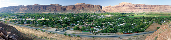
This tutorial presents a workflow for reprojecting a US Geological Survey (USGS) DEM in decimal degrees from geographic to universal transverse Mercator (UTM) coordinates. The sample dataset is the same elevation raster used to calculate slope impedance for “Creating and Deploying a Multimodal Emergency Response Network,” a companion tutorial in this issue.
In this exercise, you will learn how to reproject the source USGS data into a standard projected system and experiment with two slightly different resampling techniques. When you have looked at both methods, you can decide which you prefer.
The USGS and other federal and state elevation data providers often post DEM data in an ArcGIS grid format, applying geographic (decimal degrees or longitude-latitude) coordinates. The preferred datum is North American Datum of 1983 (NAD83). Elevation is typically reported in meters.
To analyze raster elevation data and display digital topography in three dimensions, it may be desirable (or even necessary) to reproject data to a local projected coordinate system such as UTM or state plane. Occasionally, a significant datum transformation is also required.
For many years, ArcGIS users have “reprojected” elevation and other rasters by assigning the desired coordinate system to a data frame and exporting the raster using the data frame’s coordinate system instead of the source raster’s coordinate system.
Quick and Dirty: Traditional Raster Projection
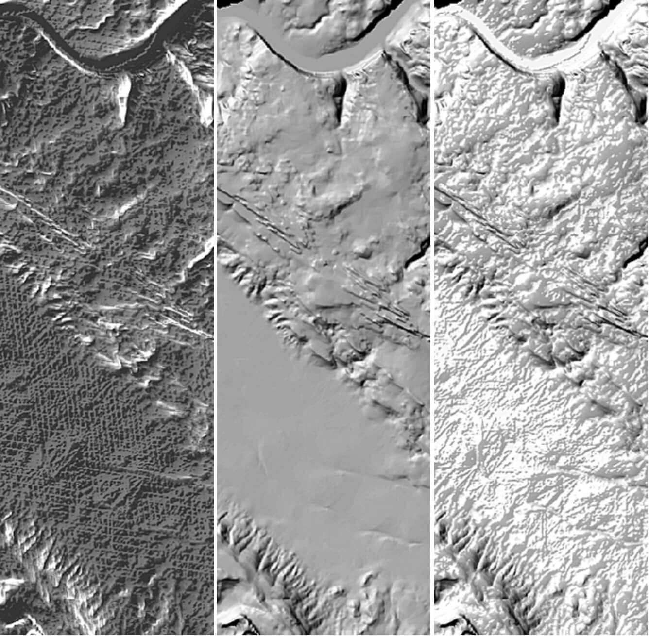
Specifying a non-geographic method for the coordinate system and exporting this raster as a new dataset to apply the data frame’s coordinate system was often ineffective, especially if the reprojection involved noticeable rotation or shearing. It applied a Nearest Neighbor resampling algorithm. Because topographic data was often inadequately resampled, a significant “herringbone tweed” artifact was created in the reprojected raster that was especially noticeable in hillshades, hydrologic flow networks, or image drapes generated from that raster. For years, the fallback strategy was to keep the source DEM in its original geographic coordinate system as long as possible. However, the raster reprojection tools in ArcToolbox allow users to accurately transform elevation rasters and other grids into a new coordinate system.
Creating a Sample Contour
Begin by downloading the sample dataset for this tutorial from the ArcUser website (esri.com/arcuser). Place the sample dataset archive in a local folder and unzip it.
1. Start ArcMap and open a new map document. In the Standard toolbar, choose Customize > Extensions and verify that the Spatial Analyst extension is available. Choose Customize > Toolbar and select the Spatial Analyst toolbar to display it. Notice that this toolbar has fewer functions than it had in previous versions of ArcGIS.
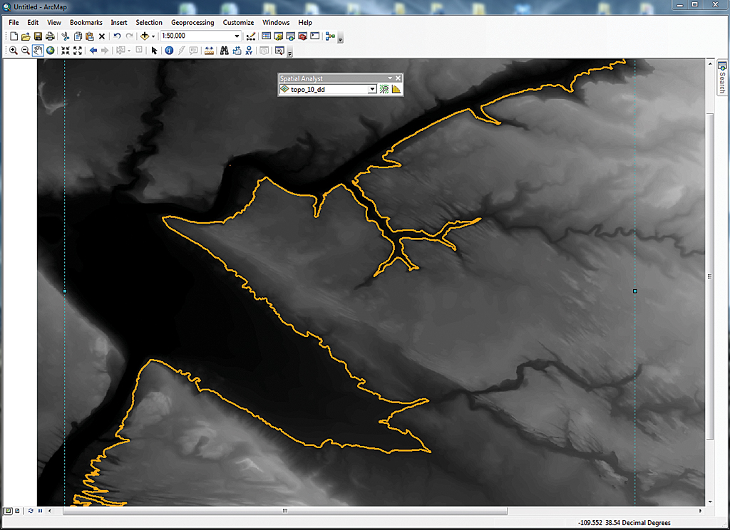
2. Click the Add Data button, go to the folder where you unzipped the sample dataset, and navigate to the \Slickrock_Topography\GRDFiles\LonLat83 folder. Add the raster DEM named topo_10_dd. This elevation raster was clipped from a larger 10-meter DEM downloaded from the National Map website. As its name suggests, the data is registered in decimal degrees. After it loads, note the coordinate system used (shown in the lower right corner of the map canvas). It should show decimal degrees.
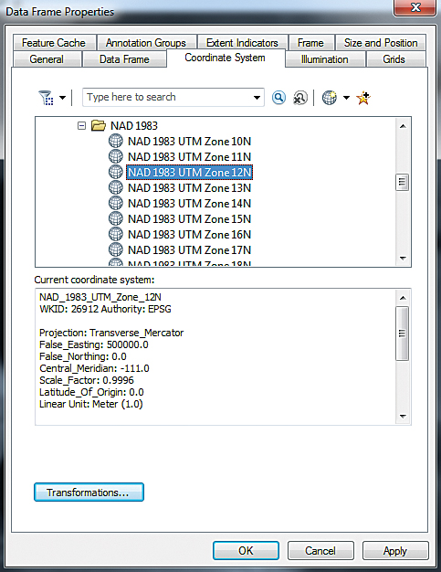
3. Open the Data Frame Properties dialog box and the coordinate system to NAD 1983 UTM Zone 12N. Because both datasets use the NAD83 datum, no datum transformation is required. Click the General tab and change the Units Display to Meters and the data frame name to NAD_1983_UTM_Zone_12N to remind you of the destination coordinate system. Close the Data Frame Properties dialog box.
4. The Create Contour tool from the Spatial Analyst toolbar will be used to create a single sample contour line to validate the elevation data. First, verify that the Spatial Analyst toolbar shows topo_10_dd as the current raster. The dark northwest trending area in the DEM is Moab Valley. Select the Create Contour tool and click the rim to the right of the valley floor. A sample contour should appear shortly. If necessary, change the contour line’s color for maximum visibility by right-clicking on the contour and choosing Properties.
5. This contour line graphic uses geographic coordinates in NAD83. Leave this line graphic in your map and save the map as SR_Topography.mxd.
Reprojecting the Right Way: Reprojecting Rasters with ArcToolbox
The ArcGIS toolbox provides a much better method for projecting rasters into a new coordinate system. In previous versions of ArcGIS, when raster topographic data was exported to a new coordinate system, the NEAREST (Nearest Neighbor) technique was used by default, which often caused problems. ArcGIS now provides four choices: BILINEAR (bilinear resampling), CUBIC (cubic convolution), NEAREST, and MAJORITY (majority algorithm). The BILINEAR option and the CUBIC option are most appropriate for continuous data, such as this floating-point topography raster. The NEAREST and MAJORITY options are used for categorical data such as a classified integer grid. ArcGIS help provides additional information on these sampling techniques.
Which technique to use, BILINEAR or CUBIC? After consulting Esri Technical Support, I learned that the bilinear resampling algorithm will smooth the continuous raster within the pixel range without extrapolating values. The CUBIC (cubic convolution) algorithm will follow a curve method and might interpolate pixels slightly above or below their source values.
Try both techniques and name each output raster accordingly. The BILINEAR output will be named utmB, and the CUBIC output will be named utmC. By trying both, you can assess just how much smoothing is acceptable or desirable for this topographic dataset; you can let contour lines help you decide.
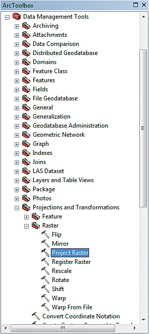
1. Add ArcToolbox to the map document and navigate to Data Management Tools > Projections and Transformations > Raster. Open the Project Raster tool. Stretch the dialog box out completely so all fields are visible.
2. Click the drop-down next to Input Raster and choose topo_10_dd. Notice that the Input Coordinate System is GCS_North_American_1983.
3. On the Output Raster Database line, click the Browse button and navigate to Slickrock_Terrain\GDBFiles\UTM83Z12. Open the SR_Terrain file geodatabase and save the file as a raster dataset with the name topo_10_utmB. Click Save but not OK.
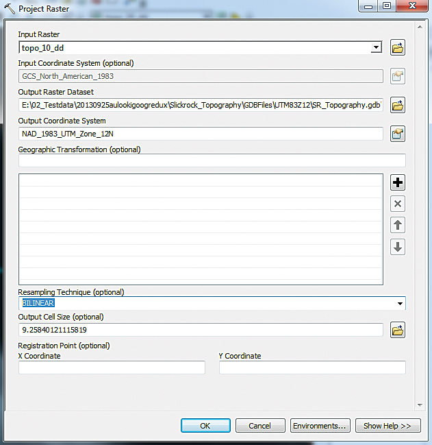
4. For Output Coordinate System, choose Projected Coordinate Systems > UTM > NAD 1983 > NAD 1983 UTM Zone 12 N. Click OK once.
5. Click the Resampling Technique drop-down and choose BILINEAR (hence the “B” in the file name). Although the dialog box indicates this is an optional step, it is not optional. Now click OK to reproject this DEM. It will be added to the map.
6. Reopen the Project Raster tool. Select topo_10_dd as the Input Raster. On the Output Raster Database line, click the Browse button and navigate to Slickrock_Terrain\GDBFiles\UTM83Z12. Open the SR_Terrain file geodatabase. This time, save the file as a raster dataset with the name topo_10_utmC. Click Save but not OK.
7.For Output Coordinate System, choose Projected Coordinate Systems > UTM > NAD 1983 > NAD 1983 UTM Zone 12 N. Click OK once.
8. Click the Resampling Technique drop-down and choose CUBIC. Now click OK to reproject this DEM. It will be added to the map.
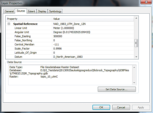
9. Check out the layer properties for each raster to verify that each has been reprojected. Save the map document.
Challenge Exercises
If you want to test these methods further, reproject the original deographic DEM using the old Data > Export procedure or reproject it using the Nearest Neighbor technique. Use the Contour with Barriers tool, located in the Surface toolset of the Spatial Analyst toolbox to create topographic contours for these reprojected DEMs and compare your results.
In most cases, you will see that these earlier, simpler methods, based on the Nearest Neighbor algorithm, behave identically and do not properly reproject the data. To really see the difference, create and compare hillshades for all reprojected topography rasters. You will see why the undesirable Nearest Neighbor artifact is called herringbone tweed.
Summary and Acknowledgments
In this brief exercise, you learned how to properly reproject a digital topography grid using two resampling techniques. These techniques will work for other continuous and categorical rasters, so try them out with your own data. When acquiring background information for this aticle, the Esri Technical Support staff helped me better understand the raster resampling algorithms used by ArcGIS.