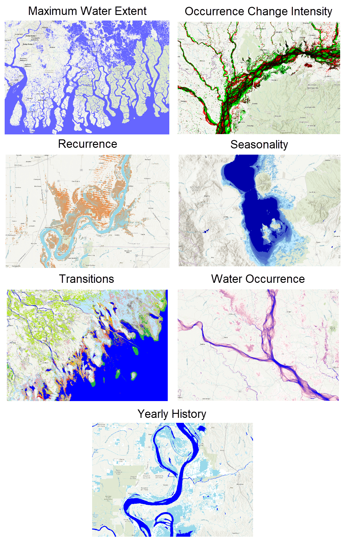
Surface water is one of Earth’s most dynamic natural resources. Rivers migrate across floodplains, reservoirs fill and empty, wetlands expand and contract with seasonal cycles, and lakes respond to both climate variability and human activity. Understanding these changes requires more than individual satellite images—it requires a consistent record of observations spanning decades.
Seven Analysis-Optimized JRC Global Surface Water imagery layers are now available in ArcGIS Living Atlas of the World, extending the global surface water record from 1984 through 2024.
Developed by the European Commission’s Joint Research Centre (JRC), these datasets use Landsat observations to characterize different aspects of the location and temporal distribution of surface water worldwide at 30-meter resolution. Ready to visualize and analyze in ArcGIS Online, the seven layers provide complementary perspectives on where surface water occurs, how persistent or seasonal it is, and how it has changed over 41 years, from individual water bodies to regional and global scales.
Explore the JRC Global Surface Water Collection
The JRC Global Surface Water collection includes seven imagery layers that characterize different aspects of surface water distribution and change. Together, these layers provide complementary perspectives on where water occurs, how persistent or seasonal it is, and how it has changed over time.
| Living Atlas Imagery Layer | What it shows |
| JRC Global Surface Water – Maximum Water Extent | Identifies locations where surface water has been detected during the observation record. |
| JRC Global Surface Water – Water Occurrence | Shows how frequently water was detected during the observation period. |
| JRC Global Surface Water – Occurrence Change Intensity | Identifies areas where the frequency of surface water has increased or decreased over time. |
| JRC Global Surface Water – Recurrence | Shows how consistently water returns from year to year. |
| JRC Global Surface Water – Seasonality | Shows the number of months per year that water is typically present. |
| JRC Global Surface Water – Transition | Identifies long-term changes between land and water states. |
| JRC Global Surface Water – Yearly History | Provides annual classifications of surface water conditions for exploring change through time. |
The layers can be used individually or together to examine surface-water dynamics from different perspectives. Because the layers share a common spatial resolution, geographic extent, and observation period, they can be combined seamlessly in ArcGIS Online to support environmental monitoring, water resource management, conservation planning, and scientific research.
Four Decades of Surface Water Change
A lot can change over four decades, and the JRC Global Surface Water collection provides a unique opportunity to visualize and analyze those changes at a global scale. From expanding reservoirs and shifting river channels to shrinking lakes and disappearing wetlands, the collection captures the dynamic nature of Earth’s surface water over 41 years of continuous observation.
One of the most striking examples is the Great Salt Lake, the largest saline lake in the Western Hemisphere. Its water levels and surface area naturally fluctuate in response to precipitation, evaporation, and inflows from surrounding rivers, but upstream water use and prolonged drought have contributed to substantial declines over recent decades. As the shoreline has receded, large areas of lakebed have been exposed, affecting wetlands, wildlife habitat, recreation, mineral industries, and nearby communities.
The swipe map below compares the Yearly Water History layer from the beginning and end of the JRC time series, illustrating the reduction in surface water extent between 1984 and 2024. This long-term perspective makes it possible to see changes in the lake’s shoreline and surrounding wetlands that would be difficult to recognize using a single image or a short observation period:
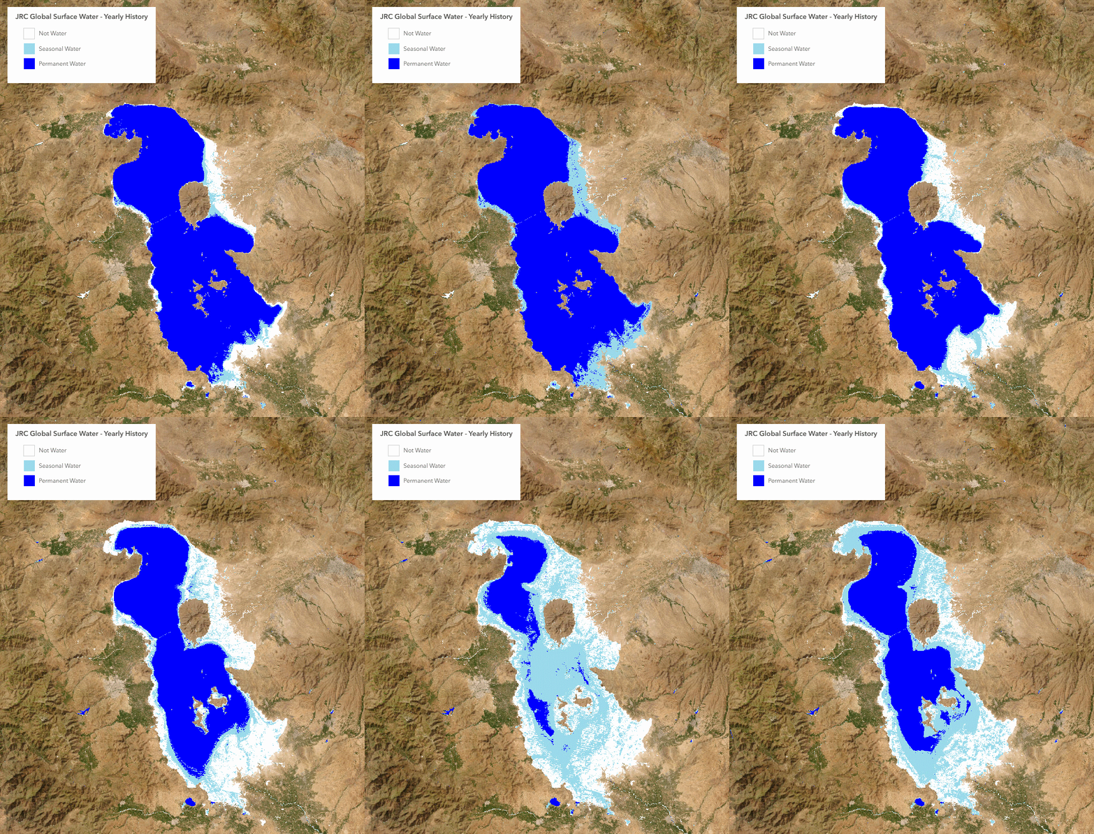
Lake Urmia in northwestern Iran provides a compelling example of how the JRC Global Surface Water Yearly History layer can reveal change through time. Once one of the largest hypersaline lakes in the world, Lake Urmia has experienced substantial changes in water extent over recent decades. Its decline has been associated with a combination of drought, agricultural water use, and dam construction on rivers feeding the lake.
The animation below follows Lake Urmia from 1984 through 2021, using the Yearly History layer to show annual surface-water conditions across the entire 38-year record. Rather than comparing only two points in time, the sequence reveals both the lake’s long-term decline and periods of temporary recovery. For example, increased precipitation in 2018 and 2019 contributed to a noticeable expansion of the lake, followed by renewed drying in subsequent years.
Viewing these changes year by year demonstrates the value of a long-term annual record: it makes it possible to distinguish persistent change from shorter-term variability and to better understand when and how changes in surface water occurred.
Processing Templates
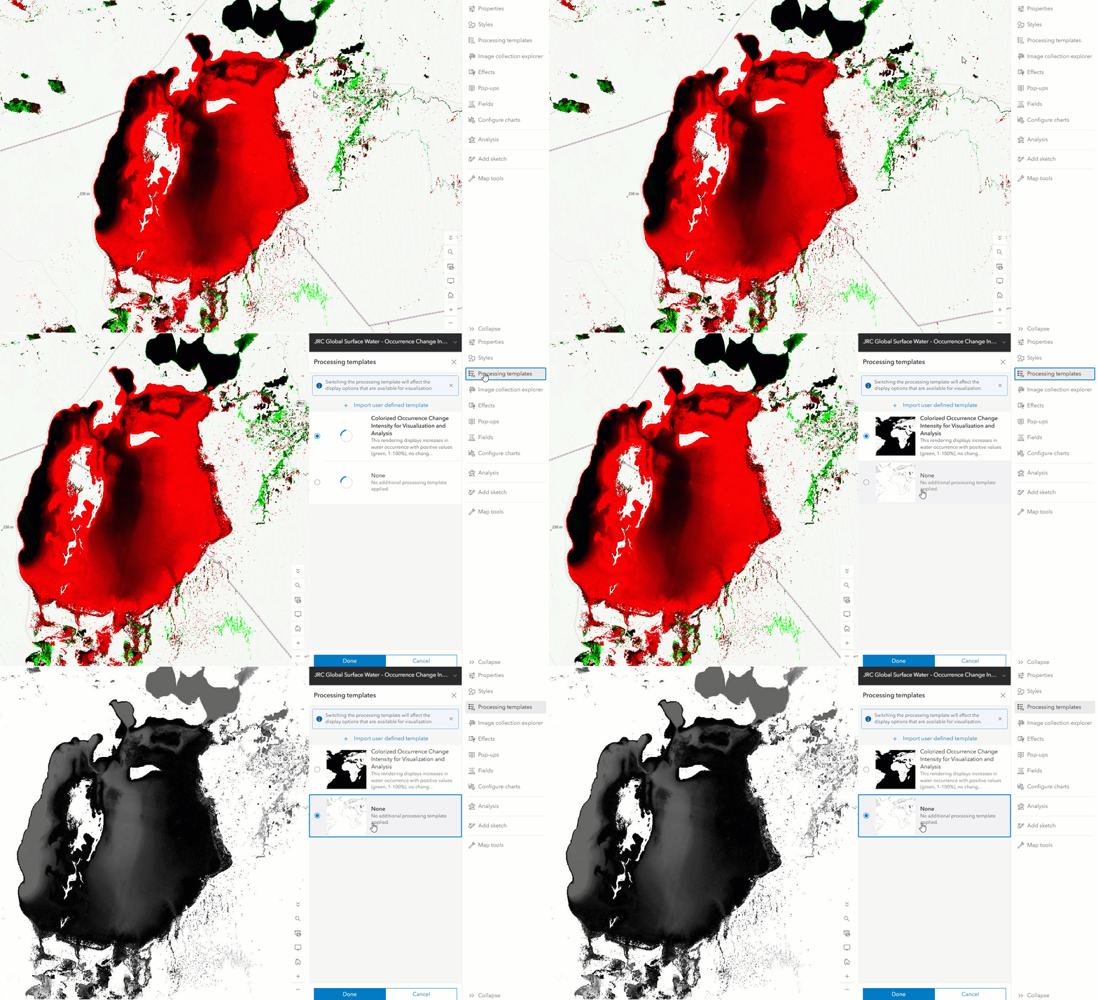
Each JRC Global Surface Water imagery layer includes two processing templates that support both visualization and analysis, providing a consistent experience across the entire collection.
The default Colorized processing template applies a predefined color ramp and rendering optimized for map visualization while preserving the raster values needed for analysis. This allows users to immediately explore the data in Map Viewer without additional symbology configuration.
The None processing template exposes the original raster values, making it easy to use the imagery as input for raster analysis, custom symbology, or ArcGIS Online raster functions. Whether you’re performing suitability analysis, overlaying other datasets, or incorporating the layers into a larger workflow, the original pixel values remain readily accessible.
JRC Global Surface Water for Optimized Analysis
While the colorized views are ideal for exploring global surface water patterns, the underlying raster values are designed for quantitative analysis.
Because these are Analysis-Optimized imagery layers, they can be used directly in ArcGIS Online with raster analysis tools such as Raster Calculator, Zonal Statistics, Classify, and other raster functions. The layers can also be combined with other Living Atlas Imagery Layers Optimized for Analysis, enabling workflows that relate long-term surface water dynamics to elevation, land cover, climate, or other environmental datasets.
Whether you’re summarizing water occurrence within watersheds, identifying areas of persistent change, or integrating multiple raster layers into larger analytical workflows, the optimized services provide scalable cloud-based analysis across large geographic extents and the complete time series.
Like other Analysis-Optimized imagery layers in ArcGIS Living Atlas, these services consume ArcGIS Online credits based on the analysis performed, while removing many of the processing limitations associated with working locally on large raster collections.

Article Discussion: