Large point datasets can tell interesting stories, but sometimes there are simply too many points to understand what is happening.
Consider 311 service requests. Across a city like Washington, DC, residents submit requests about everything from parking and traffic issues to sanitation and neighborhood services. The 311 City Service Requests in 2025 dataset contains requests submitted by the public for District of Columbia city services and information.
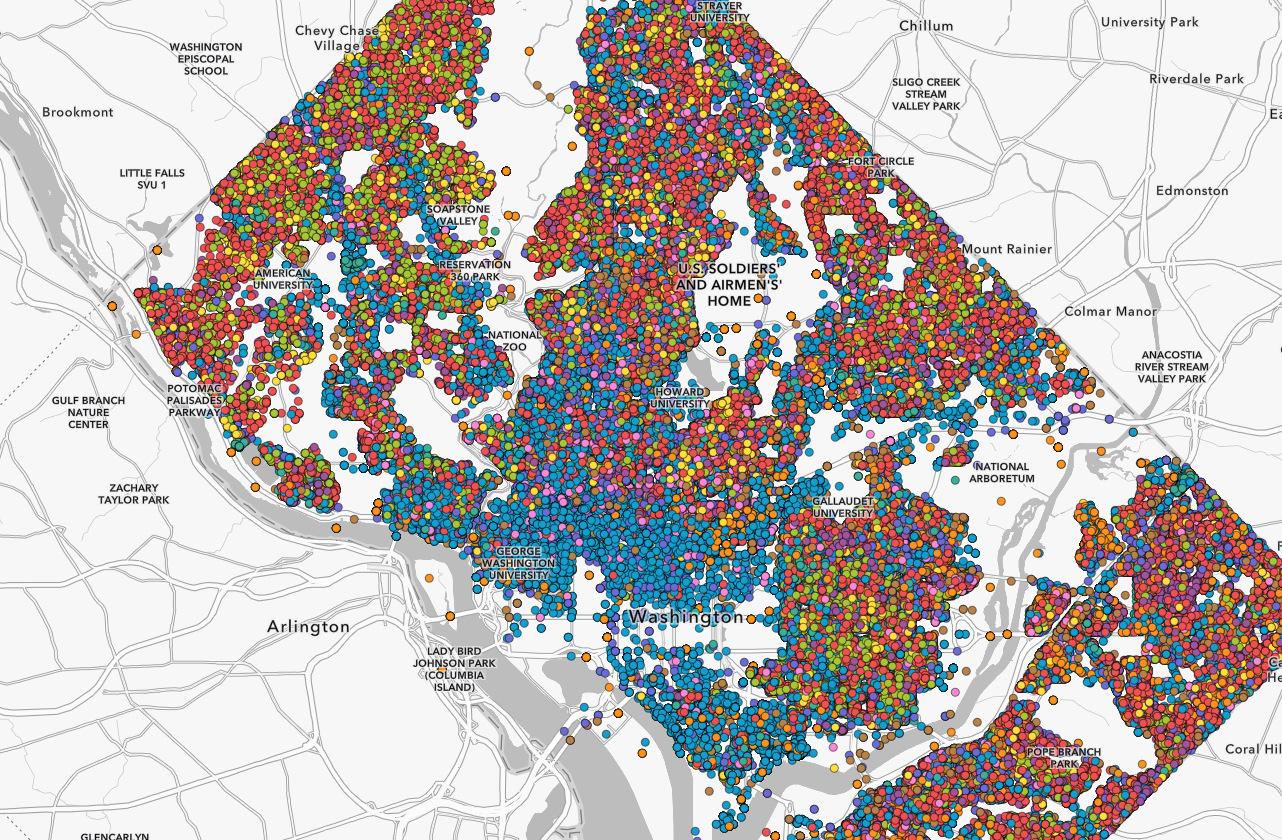
Plot those requests individually and the result can quickly become a sea of overlapping points.
Clustering provides a useful way to simplify that display by grouping nearby features together. But what if the question isn’t simply how many requests are here?
What if you want to know:
- What is the most common type of request in this area?
- How long are requests taking to resolve?
- Which parts of the city have requests taking longer than a day?
- Can we see both the type and performance of those requests at the same time?
With new cluster styling capabilities in Map Viewer, clusters can now be styled independently using aggregate attributes, summary statistics, and Arcade expressions. That turns clustering from primarily a method for reducing overlapping points into a way of exploring patterns within the features represented by each cluster.
Let’s explore what that means using 311 service requests.
Start with the points
When we first add the 311 layer to the map, each service request is represented by an individual point. At neighborhood scales, that’s useful. You can see individual requests and interact with their attributes. Zoom out, however, and thousands of individual symbols begin competing for the same space. This is exactly the kind of dataset where clustering becomes useful. When clustering is enabled, nearby requests are dynamically grouped into cluster symbols. By default, their size helps communicate the density of features as you navigate the map. But that’s only our starting point.
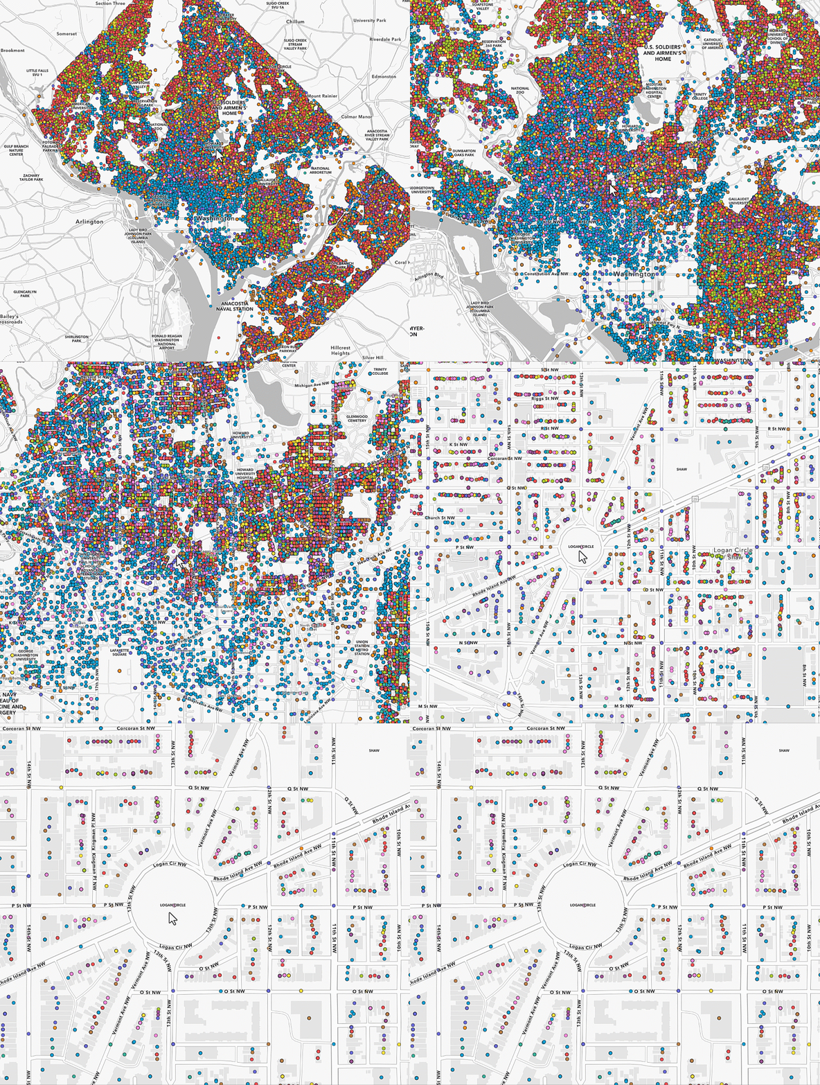
Clusters can tell you more than “how many?”
A cluster represents a collection of features, which means we can calculate information about those features.
Map Viewer lets you create cluster fields based on summary statistics and use those fields when styling clusters. Cluster styling can also use Arcade expressions, providing additional control over how aggregated information is calculated and represented.
For the 311 data, that opens up some interesting possibilities.
We might calculate:
- predominant service-request type
- average resolution time
- total requests
- percentage of requests resolved within a target period
- average or maximum response duration
Instead of asking Map Viewer only to show us where 311 calls are concentrated, we can begin asking questions about what is happening inside those concentrations.
What kind of request dominates each cluster?
Let’s start with a categorical question:
What is the predominant 311 service-request type within each cluster?
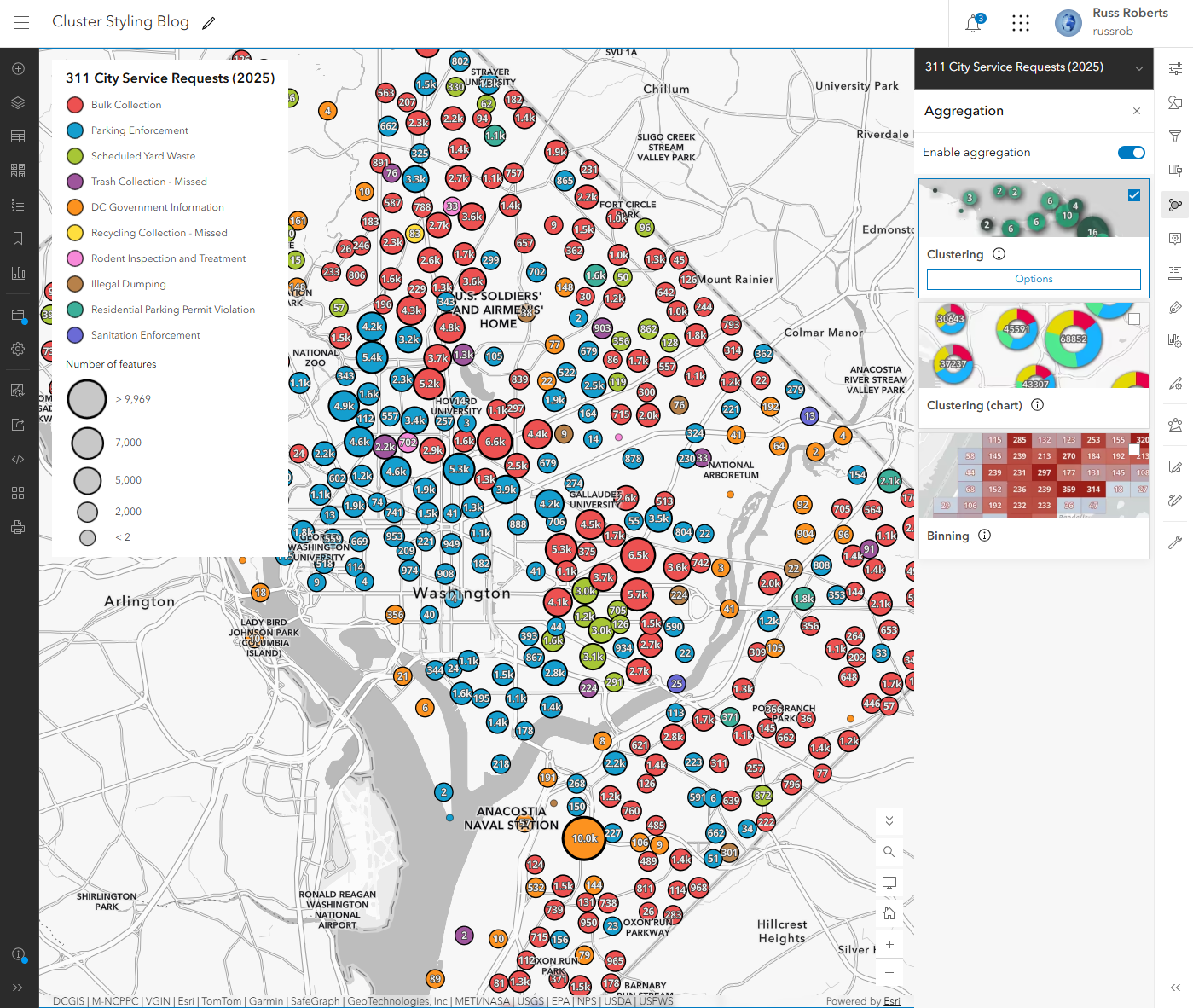
We can create a cluster field representing the predominant value of our request-type field and use that field to style the cluster.
Now color isn’t simply decorative.
Each color represents the type of request occurring most frequently among the features aggregated into that cluster.
As we move around Washington, patterns that were difficult to recognize among thousands of individual points begin to emerge.
One neighborhood may be dominated by traffic-related requests, while requests for a completely different city service may characterize another.
This is possible because the cluster renderer can be driven separately from the renderer used for the underlying features. The Map Viewer team specifically designed the new workflow so aggregated fields can drive cluster styling independently.
How long are requests taking to resolve?
Now let’s ask a different question.
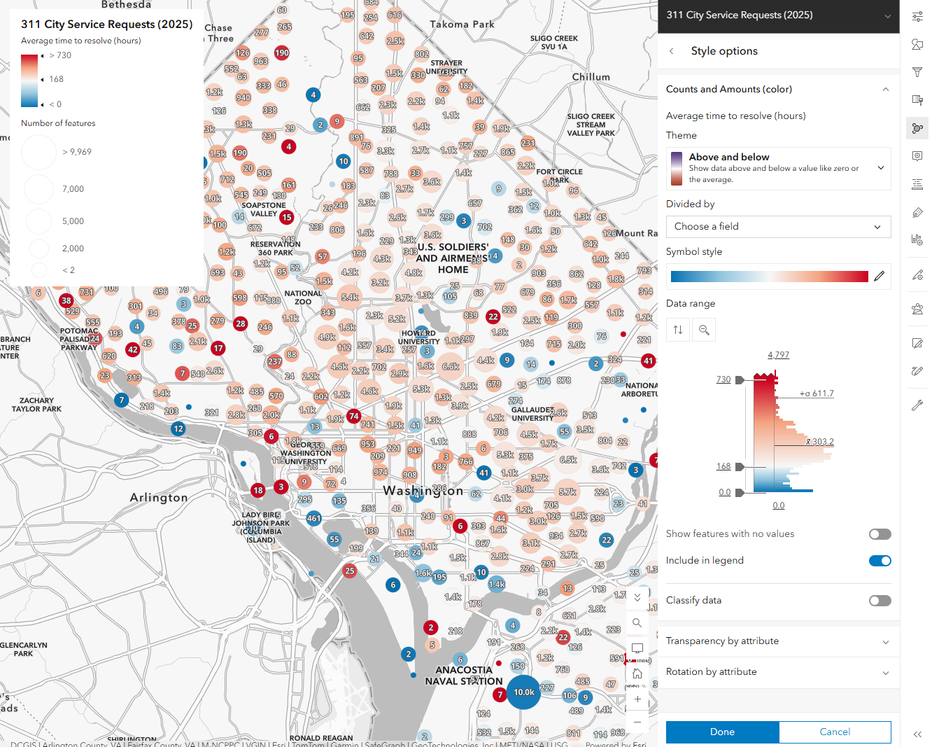
Each 311 request contains information that allows us to compare when the request was created with when it was resolved. Using an Arcade expression, we can calculate the elapsed time in hours and aggregate that information for the requests represented by each cluster. For my example, I used average resolution time. That gives us a new numeric attribute for each cluster to use for the cluster styling, popup and labels.
On average, how many hours did requests represented by this cluster take to resolve?
Map Viewer can use summary-statistic fields based off of the underlying feature fields or you can use Arcade to do more complex calculations and use them for styling. This is one of the key differences in the new experience. The cluster renderer is no longer limited to the automatically generated cluster attributes.
Suddenly, our clusters aren’t showing concentration and predominant service request. They’re summarizing service-request outcomes.
Giving time more meaning
The next step is where the visualization becomes particularly useful. Instead of applying a generic high-to-low color ramp to average resolution time, we can style the values relative to something meaningful. For this example, I used the average time field with an Above and Below theme and set the handles on the histogram to focus on 1 week(168 hrs) and then 1 month (730 hrs). The map immediately separates clusters where the average request was resolved in less than one day from those where the average went beyond one day.
Less than one day or more than one day?
That is much easier to understand. And it illustrates an important cartographic idea: a good numerical visualization isn’t always about finding the statistical middle of a dataset. Sometimes the most useful center value is one that has meaning to the person reading the map.
Now add the “what”
Average resolution time tells us how long.
Predominant request type tells us what.
The interesting part begins when we use both.
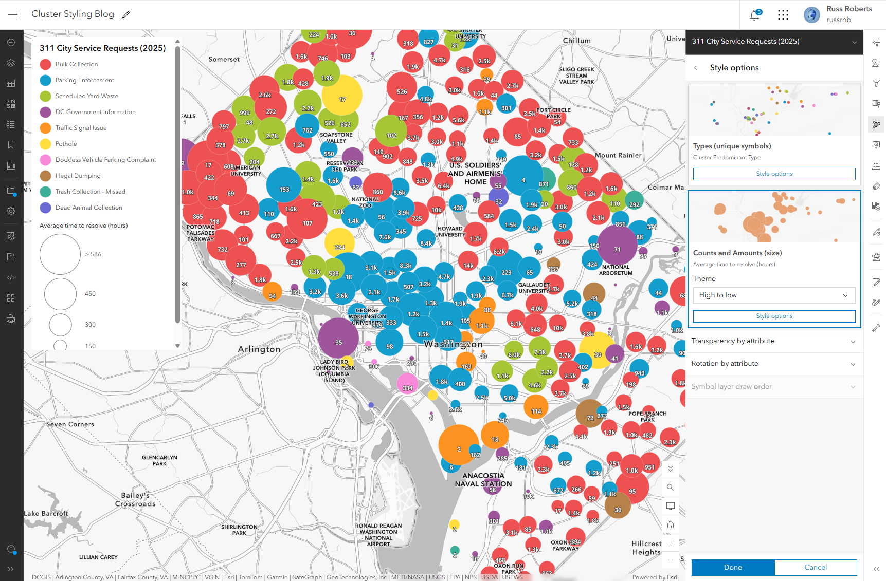
Cluster styling can combine multiple aggregate attributes in the same visualization. Internally, the Map Viewer team demonstrated this pattern with one aggregate attribute controlling cluster identity and another driving its size.
Our 311 map can apply the same idea.
For example:
Category or symbol: predominant request type
Size: Average time
The cluster stops being just a circle with a number inside it. It becomes a compact summary of the requests within that area.
Patterns emerge
This is where exploring the 311 dataset becomes particularly interesting. In the map used while testing this workflow, many of the clusters falling below the 24-hour threshold were dominated by vehicle and traffic-enforcement-related requests. Other predominant request types like potholes frequently had average resolution times extending into multiple days . That’s exactly the kind of pattern that is difficult to discover by looking at thousands of individual requests.
Build statistics specifically for your map
Not every useful statistic will already exist as a field in your layer. That’s why cluster fields are an important part of this workflow. You can create summary statistic fields from existing attributes and use those values in multiple ways. There is also the option to create more specialized arcade expressions if needed within the styling, popups and labels.
Use Arcade when the question isn’t already in the data
Sometimes the attribute you need doesn’t exist directly in the source data. Our resolution-hours example is a good case. We don’t necessarily need to modify the original 311 dataset and permanently add another field simply to test the idea. An Arcade expression can derive a value from existing attributes and use that calculation as part of the aggregation and styling workflow. This is particularly helpful during exploration. You can ask a question, create a calculation, visualize it, and decide whether the resulting pattern is actually useful before changing your underlying data model. The cluster-styling work was explicitly designed to support both summary-statistic fields and Arcade-driven calculations.
What happens to cluster size?
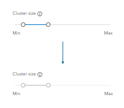
There is one subtle but important part of the new experience.
Normally, Map Viewer automatically varies cluster size according to feature density and the current map scale. But when you choose a size-based smart mapping style, such as Counts and Amounts (size) or Types and Size, size now has an explicit meaning based on the attribute you’ve chosen. In that situation, the size range defined by the style determines cluster size instead of the automatic cluster-size setting. The regular Cluster size control is disabled while the size-based style is active.That behavior matters because otherwise one visual property would be trying to communicate two different things.
With automatic cluster sizing:
Size ≈ feature density
With an attribute-driven size style:
Size = the aggregate value you’ve selected
That makes it important to decide what you want size to mean before building a multivariate cluster map.
Individual features stay part of the story
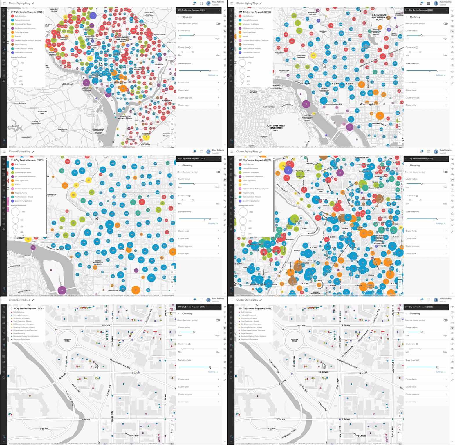
Clustering is dynamic. As you zoom into the map, clusters separate and eventually individual requests become visible again. When cluster styling is configured, those individual features can maintain visual consistency with the cluster renderer rather than suddenly switching to an unrelated styling scheme. Internally, the team described these as individual features that follow the cluster renderer, rather than exposing the implementation concept of a “cluster of one” to users.That makes the transition from overview to individual request feel like one continuous visualization.
At the city scale, you’re looking for patterns.
At the neighborhood scale, you can investigate the requests behind those patterns.
Clustering has always been useful for answering:
Where are there lots of points?
With independent cluster styling, the more interesting questions become:
- What do the points inside those clusters have in common?
- How are those groups different?
- Which category dominates?
- Are their values above or below a meaningful threshold?
For the 311 City Service Requests in 2025 data, that means we can move from seeing concentrations of requests to exploring the types of requests and how their resolution times vary across Washington, DC.
And we can do it without losing access to the individual requests that make up those patterns. That’s a significant change in how clustering can be used in Map Viewer. It isn’t just a way to clean up a busy point layer anymore.
It’s another way to explore your data.

Article Discussion: