Starting from ArcGIS Pro 3.2, the Forest-based Classification and Regression tool was renamed as Forest-based and Boosted Classification and Regression, and the tool is now able to construct not only the Forest-based model based on the Random Forest method but also the Gradient Boosted model based on Extreme Gradient Boosting (XGBoost) algorithm developed by Tianqi Chen and Carlos Guestrin. We added the Gradient Boosted model to respond to users’ requests as the XGBoost algorithm has gained popularity in recent years and is now a widely used machine learning algorithm.
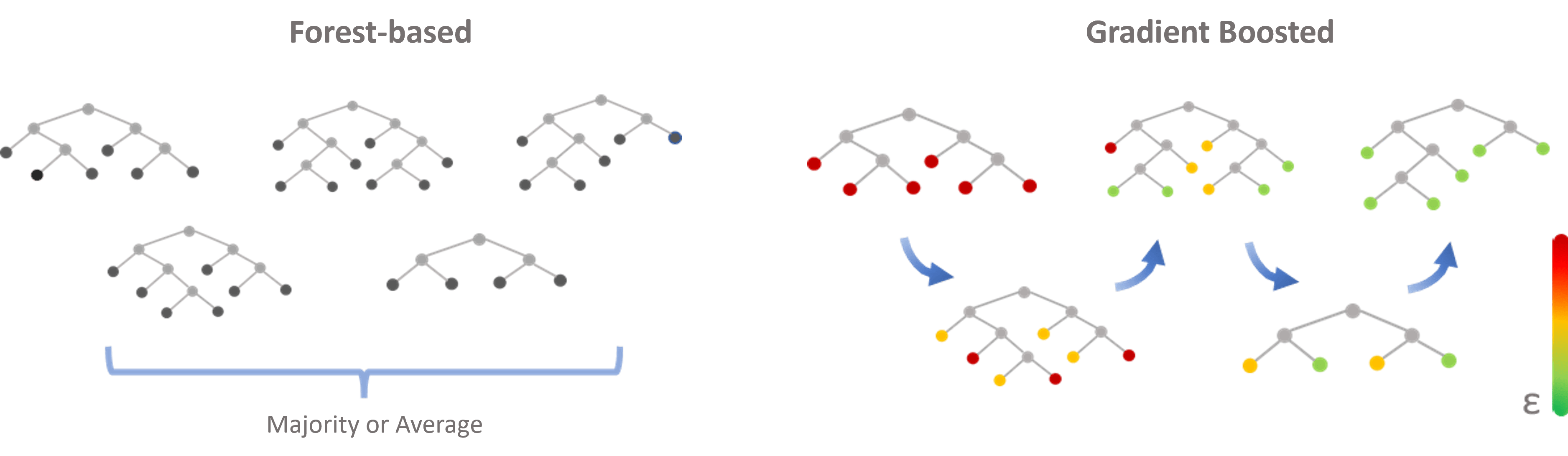
The Forest-based model and the Gradient Boosted model are both supervised machine learning models and are composed of hundreds of decision trees. However, unlike the Forest-based model in which the decision trees are created in parallel and the final predictions are generated from summarizing the independent predictions of each tree, the Gradient Boosted model builds trees sequentially, and each subsequent tree corrects the errors of the previous trees to generate the final prediction. See the illustration below. (Fig. 1)
In addition to the new model type added to the tool, now the Forest-based and Boosted Classification and Regression tool incorporates Hyperparameter tuning (Parameter optimization). Parameter optimization is important for machine learning models since the performance of the model is heavily impacted by the values of the parameters used. If we are unsure of what value to use for a hyperparameter, parameter optimization helps us to find the best value for each hyperparameter based on the criteria we specify. Now, our tool supports three optimization methods including Random Search (Quick), Random Search (Robust), and Grid Search.
In this Blog article, I use diabetes prediction as an example. With the help of parameter optimization, I will use health data to demonstrate how to construct a Gradient Boosted model. I will then show you how to evaluate the model, explore the importance and contributions of different variables, and predict the prevalence of diabetes.
Data used in this Blog Article
- PLACES, Local Data for Better Health. PLACES is a collaboration between CDC, the Robert Wood Johnson Foundation, and the CDC Foundation. The health data used in this article is a feature layer published at:
- PLACES: Local Data for Better Health (36 chronic disease)
- PLACES: Local Data for Better Health (29 chronic disease)
- Additional fields are added by applying Enrich Layer (Business Analyst) tool
Build a Gradient Boosted Model
Diabetes is a chronic disease that affects millions of people in the US, and its prevalence is a serious risk to health in Texas. According to a CDC report, there are 2.8 million cases among 29 million people in Texas. In this section, I am trying to help the state government predict diabetes at the census tract level by building a Gradient Boosted model. A model like this could help increase understanding of disease prevalence and inform the allocation of limited health resources to promote early prevention.
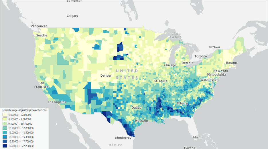
I have health data for every county from 49 states in the US (Florida is not included due to missing data) (Fig. 2). Assume that all the health-related variables that I have collected are the key factors of diabetes. These include rates of binge drinking, high blood pressure, coronary heart disease, smoking, physical inactivity, obesity, sleep quality, mobility, disability, age, frequently eating sweets, and seeking information about a healthy diet. Now, I can easily build a Gradient boosted model based on the XGBoost algorithm with the Forest-based and Boosted Classification and Regression tool.
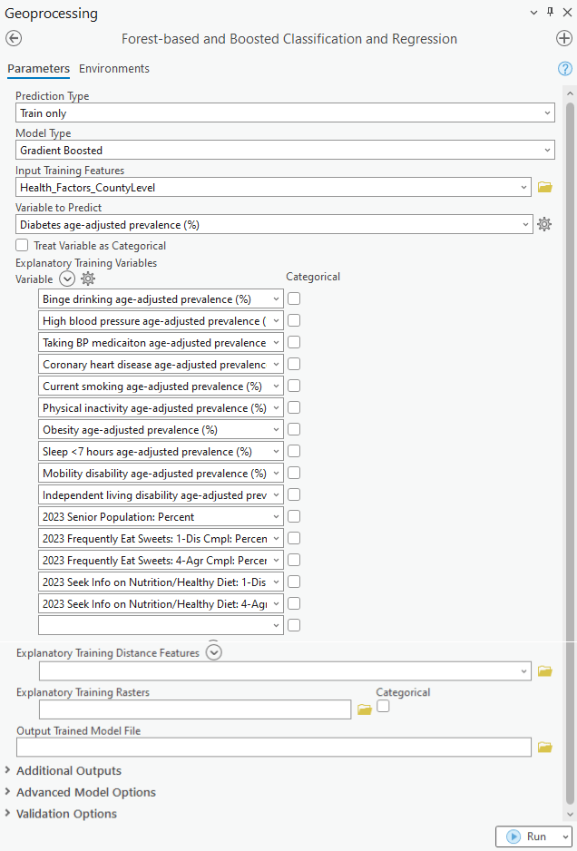
The process is very similar to how we would build a Forest-based model with this tool. The only difference is a new parameter called Model Type, where we can select to build either a Forest-based or Gradient Boosted model. To build a Gradient Boosted model, the parameters I specified are shown in the screenshot below. (Fig. 3) The Prediction Type is first set to Train because we need to assess the performance of the model before applying it to prediction. The 15 explanatory variables used are: 1) Binge drinking prevalence (%), 2) High blood pressure prevalence (%), 3) Taking BP medication prevalence (%). 4) Coronary heart disease prevalence (%), 5) Current smoking prevalence (%), 6) Physical inactivity prevalence (%), 7) Obesity prevalence (%), 8) Sleep <7 hours prevalence (%), 9) Mobility disability prevalence (%), 10) Independent living disability prevalence (%), 11) 2023 Senior Population: Percent, 12) 2023 Frequently Eat Sweets: 1-Disagree Complete: Percent, 13) 2023 Frequently Eat Sweets: 4-Agree Complete: Percent, 14) 2023 Seek Info on Nutrition/Healthy Diet: 1-Disagree Complete: Percent, 15) 2023 Seek Info on Nutrition/Healthy Diet: 4-Agree Complete: Percent
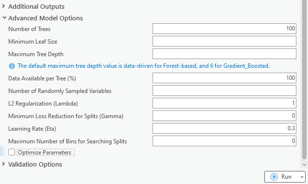
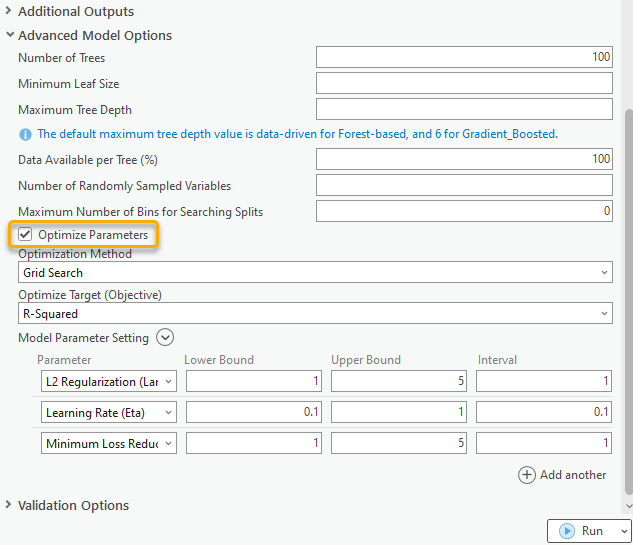
The Gradient Boosted model provides greater control over the hyperparameters than the Forest-based model. When opening the Advanced Model Options, we will notice that more parameters appear. (Fig. 4)
L2 Regularization (Lambda), Minimum Loss Reduction for Splits (Gamma), Learning Rate (Eta), and Maximum Number of Bins for Searching Splits are only available when using the Gradient Boosted model. Although there are default values and guidance on how to select a proper value for these parameters, it is almost impossible to know the best value for each of the hyperparameters.
As has been mentioned at the beginning of this article, this tool now supports parameter optimization, which tests different combinations of hyperparameter values to find the best set of hyperparameters. We can just check on the Optimize Parameter checkbox to enable this functionality. (Fig. 5) As the screenshot below, I selected the Grid Search method, which means every possible combination of parameters will be tested, and the set of hyperparameters with the best Optimize Target (Objective) score on the validation data will be used to build the model. Optimize Target (Objective) is the criteria the tool uses to determine the best values of the hyperparameters. When building a regression model, the default Optimize Target (Objective) is R-Squared. It means that the best set of hyperparameters is the value set that gets the highest R-Squared value on the validation data. In other words, the model we build can explain the most portion of the variation of the Variable to Predict. We can switch to other metrics under the Optimize Target (Objective) parameter such as RMSE if we want to find the combination of hyperparameter values which builds a model with the smallest error from the true values.
In this case, I let the tool find the best L2 Regularization (Lambda), Minimum Loss Reduction for Splits (Gamma), and Learning Rate (Eta) for me.
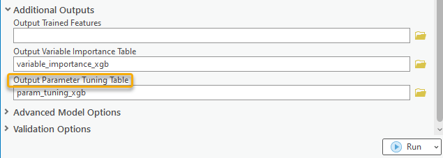
Let’s collapse the Advanced Model Options, and expand the Additional Outputs. One more parameter called the Output Parameter Tuning Table appears. (Fig. 6) I choose to save this table, so the values of the parameter combinations and objective values for each optimization trial will be exported. Additionally, two charts will be generated based on this table, which allows us to view the optimization history and the contribution of each hyperparameter to the model performance. I also choose to save the Output Variable Importance Table and hit run.
Evaluate the Model
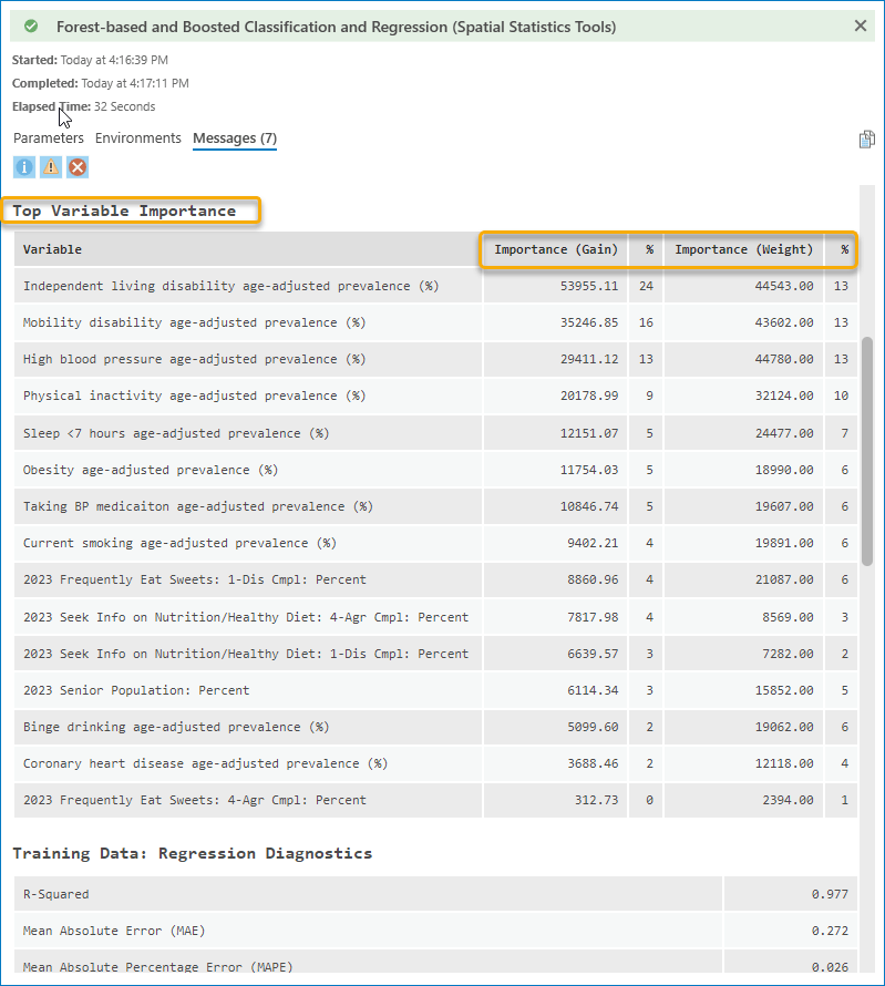
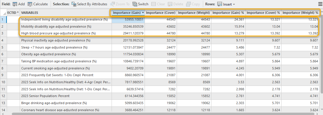
When opening the Geoprocessing Message window and scrolling down to the table, Top Variable Importance, we will find there are two types of importance listed, Importance (Gain) and Importance (Weight). (Fig. 7) Additionally, Importance (Cover) is recorded in the Output Variable Importance Table. (Fig. 8) You can check the documentation for the detailed meaning of the variable importance. We will find that independent living disability, mobility disability, and high blood pressure are the top three variables across the three different importance score calculation methods. (Fig. 8) These importance scores indicate that they are the most valuable variables when constructing this model. If we are sure that this model is good enough, we can say these three factors are highly associated with diabetes.
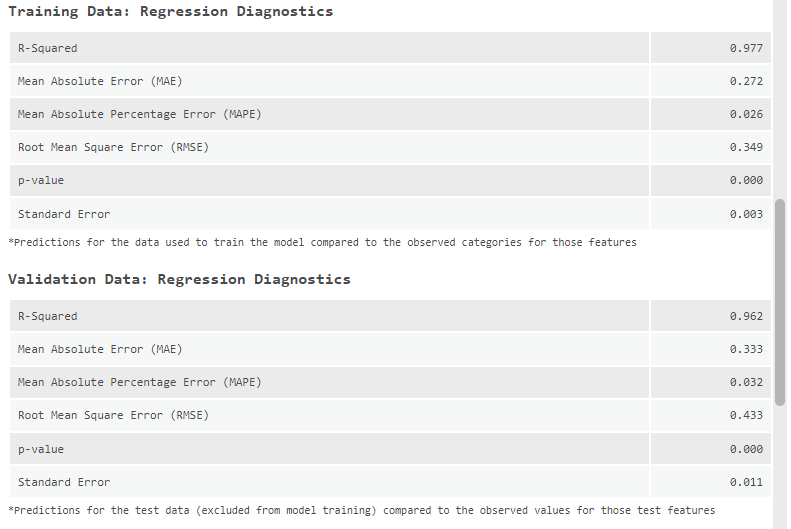
To evaluate whether it is a good model, let’s scroll down to the Training Data: Regression Diagnostics, and Validation Data: Regression Diagnostics tables. (Fig. 9) As you can see, the R-Squared score for the training data is 0.977, and for the validation data is 0.962. Three types of error (MAE, MAPE, and RMSE) are pretty low for both training and validation data. It means the performance of the model is great. The model fits very well with the training data but still does a great job on the data that the model has not seen before.
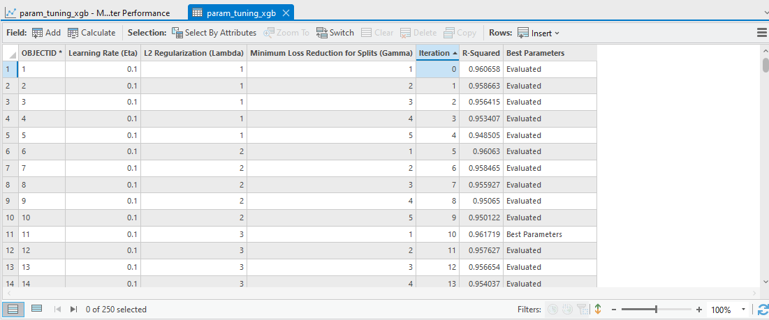
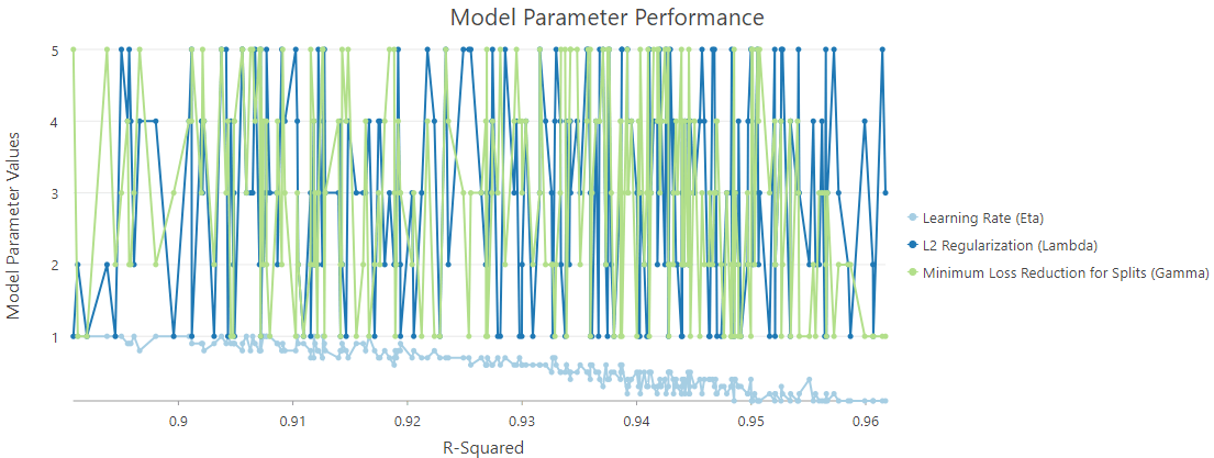
We can open the Output Parameter Tuning Table to check each optimization trial with the associated R-Squared value (Fig. 10). Furthermore, the Model Parameter Performance chart that comes along with this table enables us to explore how each parameter contributes to this model’s performance (Fig. 11).
As the chart shows, the relationship between R-Squared and L2 Regularization (Lambda), and the relationship between Minimum Loss Reduction for Split (Gamma) are not obvious. However, the relation between R-Squared and Learning Rate (Eta) is clear.
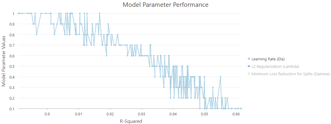
I check off other variables so that we can take a closer look (Fig. 12). The Y-axis represents the value of the Learning Rate (Eta), and the X-axis represents the R-Squared value. On this chart, a lower Learning Rate (Eta) leads to a higher R-Squared value and a better model performance.
Make the Prediction
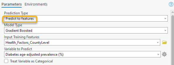
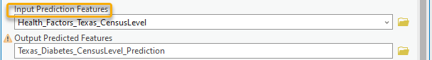
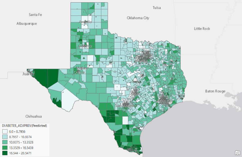
Same as the Forest-based model, once we are satisfied with the Gradient Boosted model we built, we can then apply the model to make a prediction. As shown in the screenshot below (Fig. 13 & 14), I just need to switch the Prediction Type from Train to Predict to features and provide the Input Prediction Features. Then, running the tool again will generate the predicted prevalence of diabetes at every census tract in Texas (Fig. 15).
Another way to make the prediction is to save an Output Trained Model File (Fig. 16), and use this model file as the input for the Predict using Spatial Statistics Model File tool.

Conclusion
Don’t you agree now constructing a reliable Gradient Boosted model is so much easier? The outputs, including geoprocessing messages, tables, and charts, help us evaluate the model performance and gain insight into the underlying variables contributing to the model. In addition, this tool supports parameter optimization, which enables us to easily find the best value for each hyperparameter. As Forest-based and Boosted Classification and Regression is now equipped with several powerful new features, we can’t wait to see how you will leverage this tool on your next project!

Commenting is not enabled for this article.