Understanding how long critical infrastructure like bridges will remain in good condition is a key part of risk management and resource allocation. The Estimate Time to Event tool helps us do exactly that: predict how long it will take before a bridge enters poor condition, using data and statistical modeling.
This kind of analysis can be applied broadly to infrastructure lifespan forecasting, but here we’ll focus specifically on bridges in the Pittsburgh area, using data from the National Bridge Inventory.
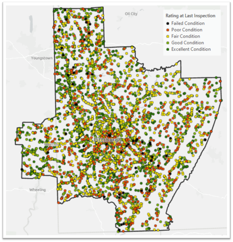
To use this tool, you first need data where the “event” has already occurred for at least some observations. For example, we need some bridges still in good condition and some already in poor condition to model how long it typically takes for deterioration to happen.
To generate predictions, the Estimate Time to Event tool requires three main inputs:
- Age of each observation (how long the bridge has been in service).
- Event indicator (whether or not the bridge has already degraded).
- Explanatory variables (factors that might influence longevity).
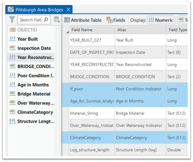
While the Bridge Inventory dataset provides lots of helpful data (some variables are shown in the Data Engineering pane below), it doesn’t give us these fields directly. We’ll need to calculate them.
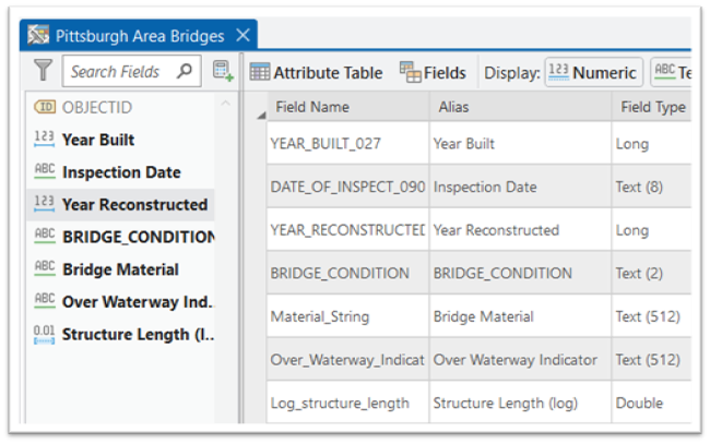
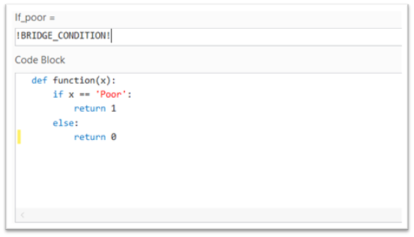
We can create a binary “event indicator” using the Bridge Condition field. For example, if the bridge is marked as Poor, we’ll classify that as a “Yes” for the event having occurred.
This transformation can be done with the Calculate Field tool. A simple function can group condition ratings and assign a value to indicate if the bridge is in poor condition.
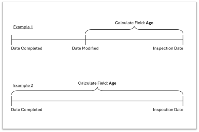
This step is a bit more involved. We’ll calculate a bridge’s age based on available dates:
- Year Completed
- Year Modified (if applicable)
- Last Inspection Date
If a modification date exists, we’ll measure the age from that date to the last inspection. Otherwise, we’ll use the original completion date (see diagram below).
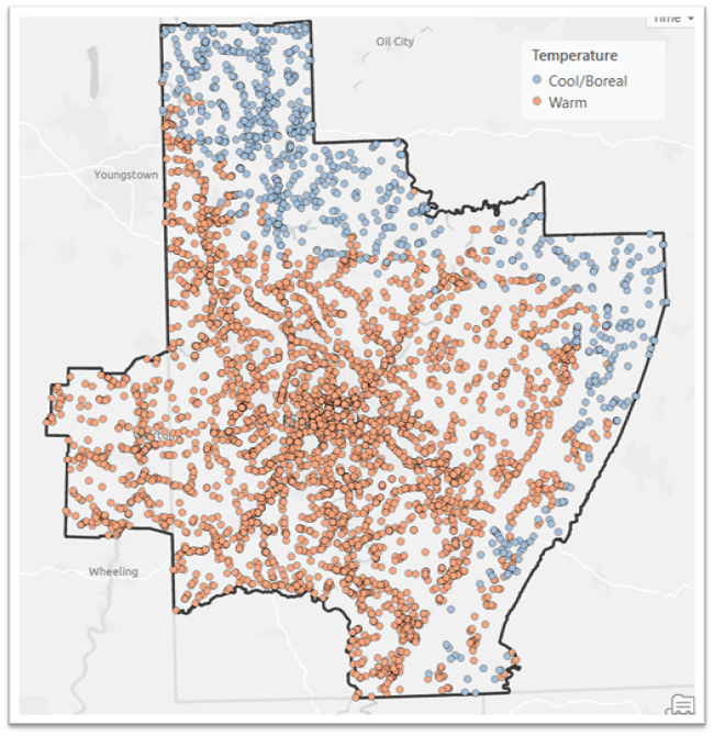
The Bridge Inventory gives us a good start, but we can enhance our analysis by bringing in additional variables. One useful example is Climate Region, available through World Terrestrial Ecosystems in the Living Atlas. Bridges in cooler areas are likely to face more degradation. The map below shows the bridge data enriched with information on the ecosystem.
Once the data are transformed and enriched, as shown in the Data Engineering pane below, we’re ready to run the Estimate Time to Event tool.
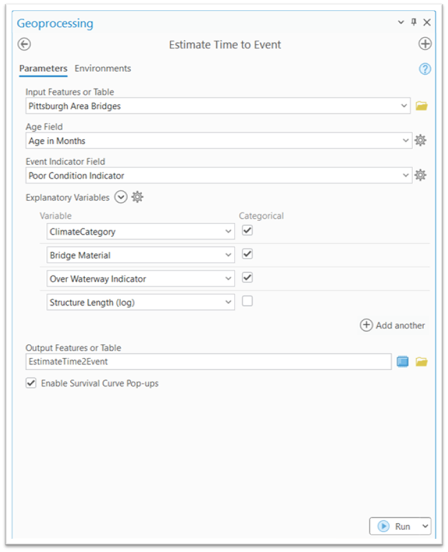
The Input Features are the Pittsburgh Bridges, the Age input is the newly calculated “Age in Months” field, and the Event Indicator is the “Poor Condition Indicator” field we created from the Bridge Condition.
The explanatory variables we will use to help us predict are:
- A binary variable indicating whether the bridge is over a waterway
- A categorical variable indicating the material of the bridge (e.g., steel, wood, etc.)
- The length of the bridge
- and the climate category variable we enriched
Once all this information is input, we can run the tool (shown below) and inspect the output.
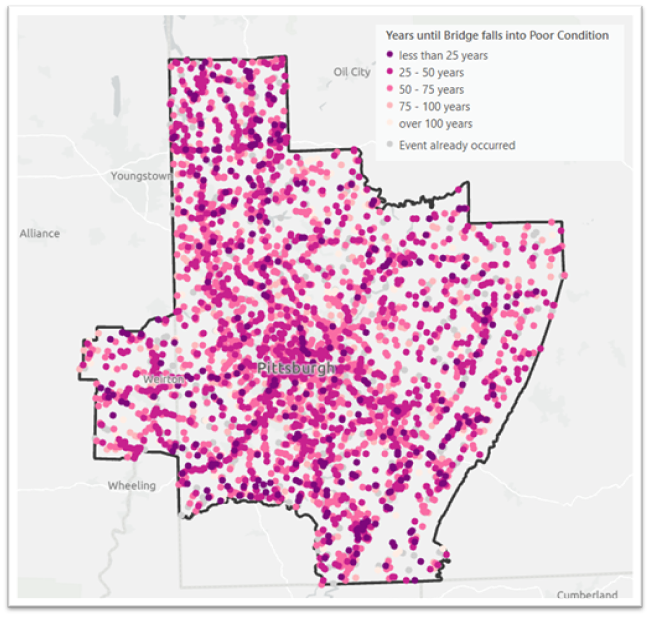
Once the tool runs, the output map below highlights which bridges are at higher risk. Bridges with shorter predicted timeframes until degradation are shown in dark purple. Some may fall into poor condition within the next 25 years.
But the tool doesn’t stop at predictions, it also provides insight into why a bridge has a shorter or longer predicted lifespan. That’s where come in:
- A Time Ratio < 1 means the variable shortens the bridge’s expected lifespan.
- A Time Ratio > 1 means it lengthens the lifespan.
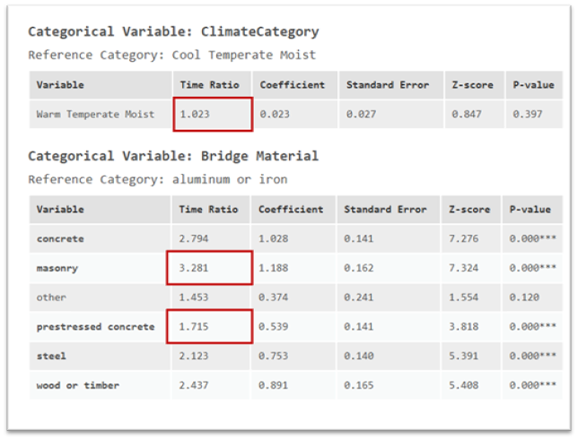
The time ratios in the output message table below tell us that, for length, longer bridges tend to have shorter predicted lifespans (the Time Ratio is less than 1).

For Climate Categories, Warm temperatures are associated with longer lifespans than the baseline, which is Cool temperature regions (the Time Ratio is greater than 1). For Bridge materials, we can learn that masonry builds tend to last longer than prestressed concrete builds (the Time Ratios are both greater than 1, but the Time Ratio for masonry is almost 2x larger). All of these material time ratios are in comparison to the reference category: aluminum and iron builds.
The New Estimate Time to Event tool opens new doors for predicting the occurrence of events in the future. This type of analysis can be used for infrastructure management, and a wide array of other problems: How much longer will this tree live? When will this customer leave my company? How long can we expect this coral reef to survive?
Learn More:
Estimate Time to Event Tool Documentation
How Estimate Time to Event Works

Article Discussion: