This might make me sound nerdish, but I am a huge fan of geostatistical interpolation methods. Among my personal favorites are Empirical Bayesian Kriging (EBK), EBK Regression Prediction, and Empirical Bayesian Kriging 3D. Now you can probably guess how excited I am about the latest update on Geostatistical Analyst in ArcGIS Pro 3.0. In this blog post I will use the opportunity to share with you a couple of new tools that we added in the Geostatistical Analyst extension, and to summarize some of my favorite geostatistical interpolation workflows.
For those of you who are not too familiar with the ArcGIS Geostatistical Analyst extension, it is designed specifically for spatial interpolation. Spatial interpolation uses measured values taken at known sample locations to estimate values for unknown locations.
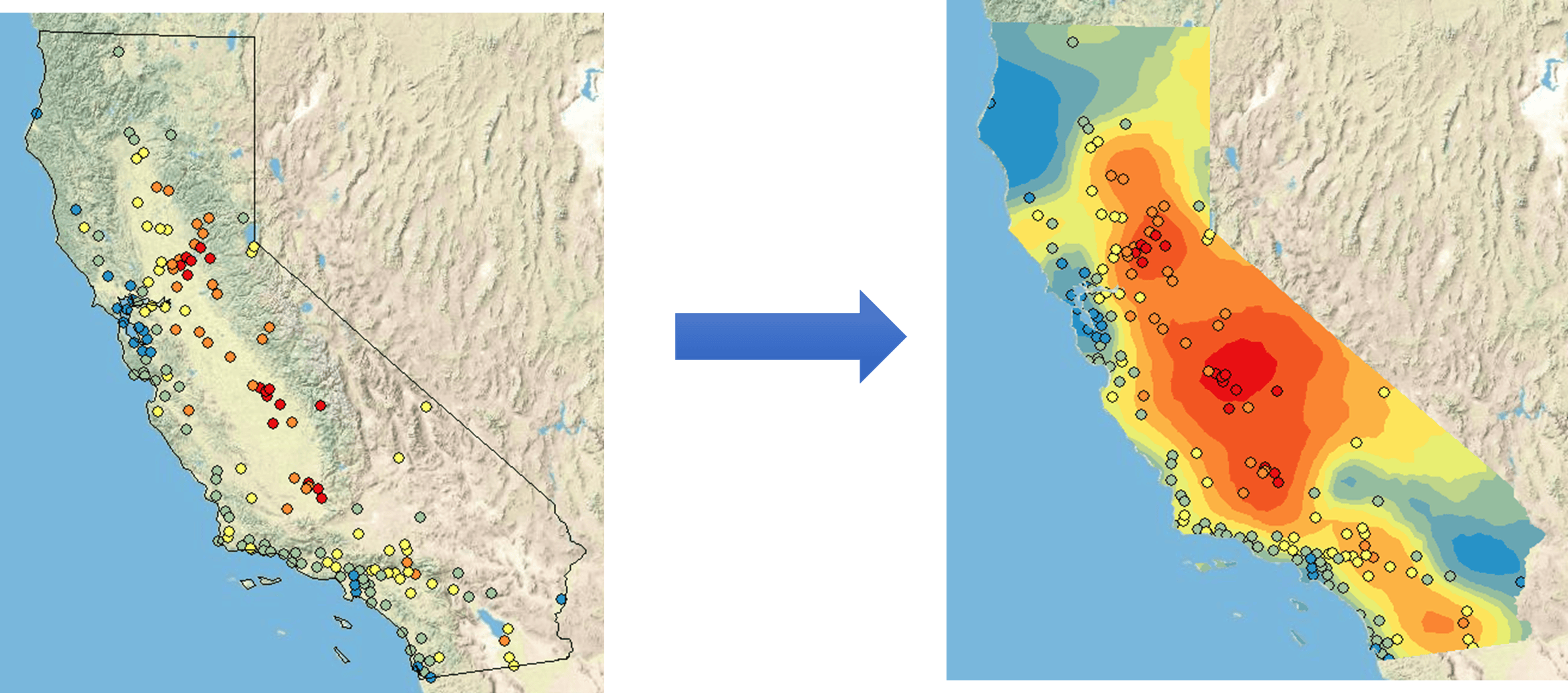
Due to cost and practicality, collecting data everywhere is not always feasible. For example, The California Air Monitoring Network consists of more than 250 monitoring stations operated by federal, State, and local agencies. In order to create a map of ozone concentrations for the entire state of California, we can use interpolation techniques to estimate ozone concentrations at locations without recorded data by using readings from the nearby sample monitoring stations. We can then produce a continuous surface of ozone concentrations based on the interpolated results.
Because spatial interpolation generates a continuous surface based on sample points, we generally recommend using it on continuous data, such as air temperature, elevation, pollution level, or an oil spill.
Spatial interpolation is based on spatial autocorrelation, which measures the similarity between nearby observations. You may have heard of Tobler’s first law of geography: “Everything is related to everything else, but near things are more related than distant things”. For example, in an elevation dataset, the neighboring cells tend to have similar or the same elevation values. The primary assumption of spatial interpolation is that the sample points used for interpolation are correlated spatially.
Spatial interpolation is one of the most common workflows in GIS. It is widely applied in many fields especially in atmospheric data analysis, petroleum and mining exploration, environmental analysis, precision agriculture, and fish & wildlife studies.
As I mentioned earlier, the ArcGIS Geostatistical Analyst extension focuses on spatial interpolation. It is designed to address questions such as: What is the value of a variable at a new location? What is the uncertainty of the estimate? The statistical models and tools available in Geostatistical Analyst help to derive accurate and reliable estimates for phenomena at locations where no measurements are available. In addition to deterministic methods such as inverse distance weighted interpolation (IDW), the most powerful interpolation tools in ArcGIS Geostatistical Analyst are based on kriging techniques. Kriging first uses semivariogram to model spatial autocorrelation of the measured sample points, then applies this model to predict values at unmeasured locations, and also assesses the uncertainty associated with a predicted value at an unmeasured location.
Traditional kriging methods involve interactive semivariogram modeling as a preliminary step, which requires experience in fitting data to a semivariogram model. In addition, there are several kriging tools to choose from, and there are different options for parameter input for each method. Therefore, performing spatial interpolation can be a daunting task. To ease this pain point for the users, it has always been one of our goals to develop a spatial statistical interpolation model with automated semivariogram modeling and smart defaults.
Empirical Bayesian Kriging (EBK)
Empirical Bayesian Kriging (EBK) in the Geostatistical Analyst extension was a game changer for having both an accurate and easy-to-use spatial interpolator. EBK uses local models to capture small scale effects, therefore, it does not assume that one model fits the entire data. As a result, it requires minimal interactive modeling. Spatial relationships are modeled automatically, the statistical assumptions are more flexible than traditional kriging methods, and the prediction accuracy is higher for large and small datasets. In addition, EBK uses smart defaults to simplify the decision process for users.
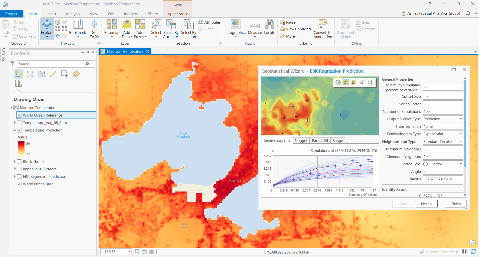
EBK Regression Prediction
Although EBK has been proven to be a straightforward and robust spatial data interpolation method, a location’s value is often not only related to the values of points nearby but also depends on other explanatory factors. For example, when interpolating temperature data, we may want to take into account the elevation data in addition to temperature readings from nearby weather stations.
EBK Regression Prediction tool combines kriging with regression analysis. It allows us to make predictions using additional explanatory variables. EBK Regression Prediction can be widely used in many applications. For example, we may want to consider road density, distance to major roads and residential areas, etc., when interpolating the noise pollution level for a city. Comparing the prediction results from EBK Regression with the results from EBK, you can see that because we had incorporated more explanatory variables in addition to the noise samples, the results look much more local and accurate, and we can pick out much more details.

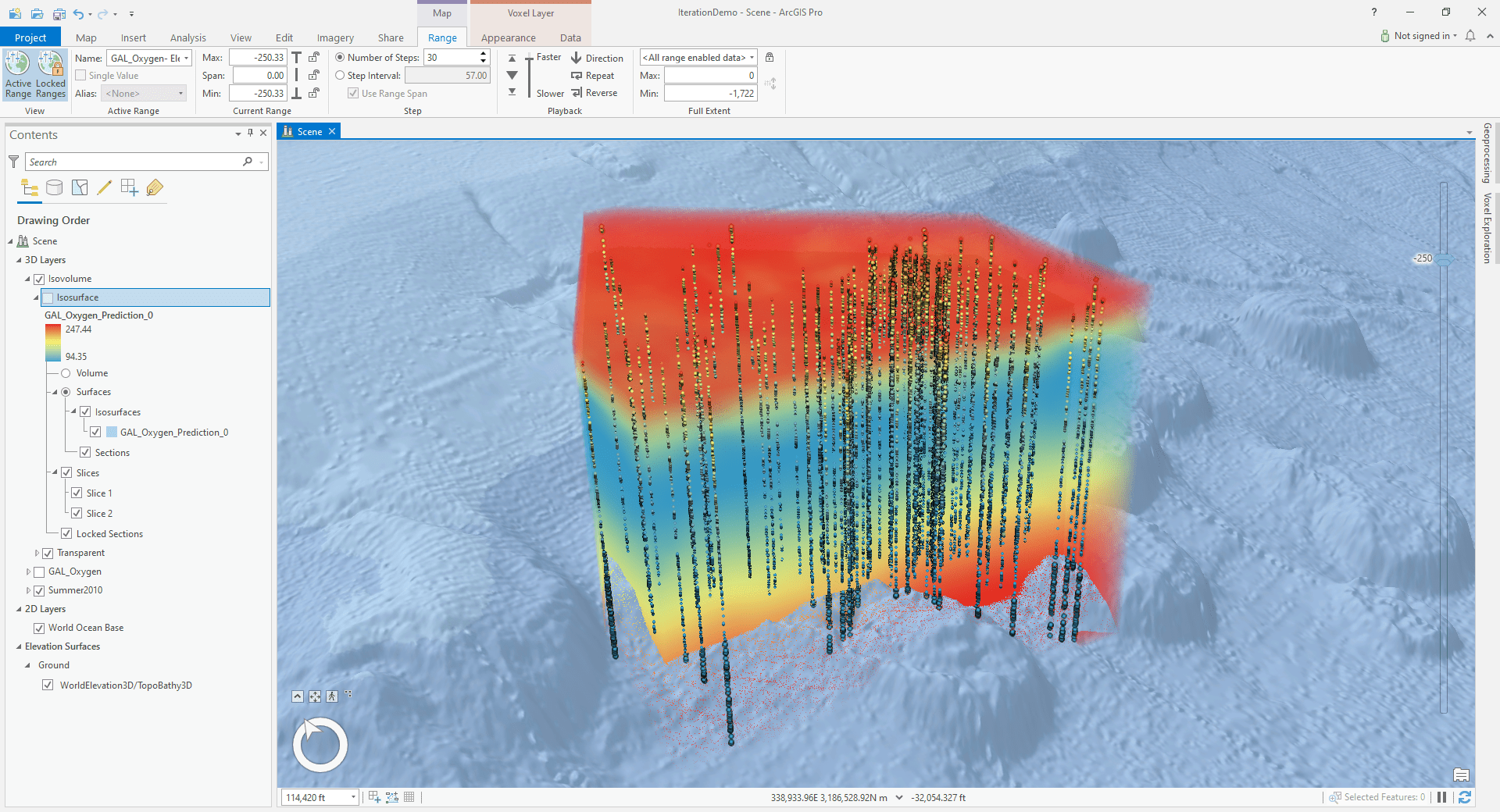
Empirical Bayesian Kriging 3D
An exciting new tool in the Geostatistical Analyst extension is Empirical Bayesian kriging 3D. This tool uses Empirical Bayesian Kriging (EBK) methodology to interpolate points in 3D space. The EBK 3D model simultaneously accounts for the different spatial correlations in the X, Y, and Z (height or depth) dimensions. EBK 3D allows you to generate prediction surfaces for natural phenomena with 3D measurements. For example, in oceanography, 3D interpolation can be used to create maps of dissolved oxygen at various depths in the ocean. Using the new Voxel layers available in ArcGIS Pro, the Geostatistical Analyst users can visualize and interactively explore the details of the 3D geostatistical layers created by the EBK 3D tools.
What’s new for Spatial Interpolation in ArcGIS Pro 3.0
As I mentioned above, one of the challenges many users face with the interpolation process is how to choose the best interpolation model. In the upcoming ArcGIS Pro 3.0 release, the Geostatistical Analyst team focuses on improving this workflow. Two new tools are added in the extension in ArcGIS Pro 3.0:
Compare Geostatistical Layers
This tool compares and ranks prediction results from various interpolation models using customizable criteria based on cross-validation statistics. It helps analysts to interpret geostatistical model results and to automate the selection process to find the most suitable prediction model.
Video Credit: Eric Krause
Exploratory Interpolation
This tool takes an input of sample points and the prediction field and generates various interpolation results based on different models. The interpolation results are then compared and ranked using customizable criteria based on cross-validation statistics. This helps ease the difficulty many users often have in choosing the best geostatistical model.
Video Credit: Eric Krause
Well, that’s all with an update on the recent developments in the ArcGIS Geostatistical Analyst extension. As always, I would love to hear your experiences and comments!

Can this method able to be implemented in Oil & Gas needs as practice, example to calculate the volume of cut and fill in swamp area?
The example you refer to is related to volumetric calculations. You might want to check out the cut fill tool in ArcGIS Spatial Analyst or ArcGIS 3D Analyst extension.
Hello, Jian and Eric. Thank you very much for the videos. I would like to know if the models generated from 3D Bayesian Kriging can be exported in such a way that they can be viewed in other programs, for example AutoCAD.