Updated June 9th, 2021: This blog was updated to reflect the enhancements of Distance Toolsets in ArcGIS Pro 2.8.
Accessibility is defined as “the quality of being easy to approach, reach, enter, speak with, use, or understand.” In context of international development, accessibility is often used to understand if residents can reach schools, health centers, infrastructure, or jobs within reasonable effort when needed. This is important to maximize outcome and ensure a more inclusive development.
GIS offers multiple approaches to evaluate accessibility. The most commonly used spatial technique to evaluate accessibility is through a network analysis. In a network analysis, a network dataset contains data about the underlying transportation network (motor vehicle roads, paths, trails, and so on), including information about speed limit, directionality, connectivity, surface type, and more. It is used to calculate how far an individual can travel in a specified time by various modes of transport, including walking and driving. You can also apply network analysis to datasets like the General Transit Feed Specification (GTFS) to determine accessibility based on public transportation schedules and their location.
While network analysis is a proven way to evaluate accessibility, its use is limited by the availability of network data. In regions with the greatest need for aid, such as sub-Saharan Africa and southeast Asia, network data is only available for major highways, which has limited use when you must calculate accessibility in rural and underserved regions. Despite these limitations, you can quantify accessibility even in absence of network dataset by applying spatial analysis to geographic features like elevation, land cover, and others.
Region names are used for managing data. They don’t necessarily correspond to the correct continent name or generally accepted regional classifications.
The conceptual approach
Before you learn how to determine accessibility using tools in ArcGIS Pro, begin with the following high-level conceptual overview of the approach.
In absence of network data, the quickest way to model accessibility is by creating a buffer around a location. For example, if you want to generate a buffer to model the distance a person can walk in 60 minutes, you can create a buffer with a radius of 2.5 kilometers, assuming an average walking speed of 5 kilometers per hour. While this may be a fair approximation in urban settings where walk time may be predictable, there are obvious limitations in rural areas. For example, the walking pace varies depending on the slope of the terrain (flat versus steep), the type of surface (pavement versus mud), and the presence of geographic barriers such as rivers, lakes, and mountain ranges.

To overcome these limitations, you can model accessibility using topography, which in part is represented by raster layers like digital elevation models (DEM). In this approach, a DEM is used to calculate the slope of the terrain, and the slope is used to determine the maximum walkable speed. For example, Tobler’s hiking function predicts that the maximum walking speed of 6 kilometers per hour is achieved at a downward slope of -3 degrees. Modeling walking speed is not limited to Tobler’s hiking function as there are other models (for example, Naismith’s rule) to predict walking speed based on slope.

Figure 1 shows Naismith’s rule – Wikipedia: https://en.wikipedia.org/wiki/Naismith%27s_rule.
You can further refine the model by introducing barriers and costs. For example, you can assume that individuals will not swim across rivers, even though crossing a river may represent the shortest physical distance from their location to their destination. In this context, you can use geographic features of rivers, which are represented as lines in GIS, and model them as barriers that cannot be crossed. You can apply the same logic to other geographic features, such as mountains, dense forests, and lakes.

A comparison of accessibility using buffer versus geographic features is shown.
In addition to introducing barriers to the model, you can also incorporate impedances. For example, not all surfaces are created equal—paved roads are easier to walk relative to dirt trails, and dirt trails are easier to walk relative to agricultural or wooded land. You can model these variances in walkable surface types through cost surfaces, which introduce impedances, or costs, to walk over the area given the nature of the walkable surface. For example, using a publicly available land cover dataset from Esri’s Living Atlas and roads data from OpenStreetMap, you can derive three surface types—roads, grassland, and forests—to represent low to high impedance, respectively. You can give each of these surfaces a numeric score (1–3) to model the relative difficulty between surfaces; 1 (one) being the easiest to walk on and thus the quickest. For example, a surface type with a value of 2 is considered twice as difficult to walk as a surface type with a value of 1.

An example cost surface shows three categories: urban/road (green), areas of minimal vegetation (purple), and forests (orange).
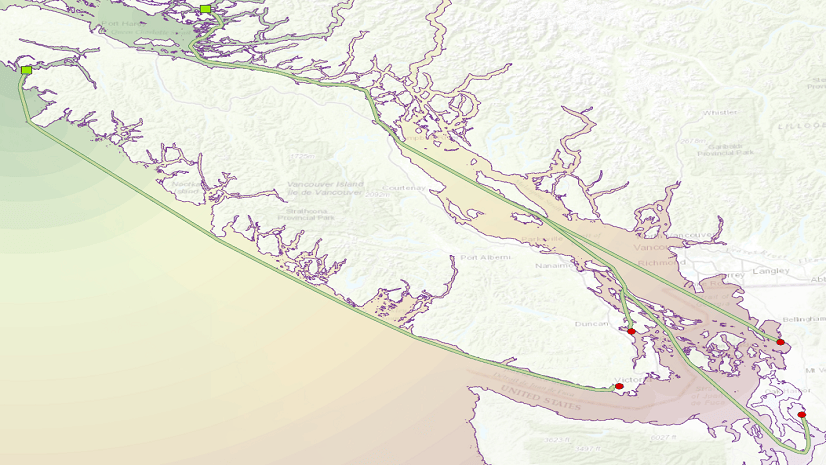
Incorporating the data layers discussed above—DEM, rivers, land cover, and roads—you can determine a walk-time distance in absence of a network dataset.

The output polygon from the model represents the outer boundary in which an individual can walk to a location within one hour.
The technical approach
ArcGIS Pro has a set of Distance tools focused on calculating paths and distances. To evaluate accessibility, you will use a tool called Distance Accumulation, which calculates accumulated distance for each cell to sources. This blog will outline the steps to evaluate accessibility based on a walk time of 1 hour.
The tool has several required and optional parameters. The following walks through each in detail.

(1) Input raster or feature source data is the location you want to evaluate for accessibility. These can be schools, health clinics, or aid distribution centers. These are represented as red dots in the image below.

The red dots represent the source feature data to evaluate accessibility.
(2) Output distance accumulation raster is the final output that shows walk-time distance from each source location.
(3) Input barrier raster or feature data represents geographic features that individuals cannot cross. This can be large bodies of water like lakes and rivers, mountain ranges, private property, or even dense forests. You must determine which natural or man-made features would act as barriers in your scenario. The input can be either feature or raster. Personally, I find raster to be more flexible as it can treat both line and polygon features (for example, rivers and lakes) as barriers in a single layer.

The blue line is a river, which represents a barrier that cannot be crossed.
(4) Input surface raster is an elevation layer (DEM). This layer is used to calculate the actual surface distance travelled when moving across cells, ensuring a more accurate output. You can use elevation layers from Esri’s Living Atlas or USGS or bring your own. Regardless of the source, the aim is to use a layer with a resolution that is appropriate for your analysis.

The gray scale raster represents elevation. Lighter the color, higher the elevation.
(5) Input cost raster represents the impedance to move through each raster cell. If input barriers represent surfaces that are impossible to cross, the cost raster represents surfaces that can be crossed but at varying difficulty. You can derive the cost, which you must define, from a single layer or incorporate multiple layers through weighted sum or overlay. For simplicity, the sample cost raster used global land cover data from Living Atlas to create three costs based on different types: urban, vegetation, and forests.
.")
An example of cost raster is shown. Each color represents a different surface type (road, agriculture, and forest).
(6) Input vertical raster uses the same elevation layer as the surface raster. The vertical factor gives you different ways to model the difficulty of moving across surfaces with changing elevation. While there are predefined models such as VfBinary, VfLinear, and others, this example uses VfTable to define a custom model based on Tobler’s hiking function. This text file (VfTable_Tobler) contains two columns to define pace at various slope with units of time/distance (for example, hours per meter). You can also explore the Microsoft Excel file (ToblerCalc) to see how the model was generated.
 is a representation of the Tobler’s hiking function (left –green line).")
The Vf_Table (right) is a representation of the Tobler’s hiking function (left –green line).
(7) Characteristics of the sources is how you further control the output model. For clarity, Travel direction is explained first followed by the Maximum accumulation, Initial accumulation, and the Multiplier to apply to costs.
(7-1) Travel direction defines the direction of travel. Because this tool uses slope to estimate maximum walking pace and the slope varies depending on the direction of travel, this parameter can impact the final output, especially in areas with variable terrain. The two options for this parameter are To_Source and From_Source. To determine accessibility of a health clinic, for example, use the To_Source parameter as patients will need to travel from their home to the clinics. On the other hand, if you want to model a scenario where staff will distribute aid in the community from a central distribution site, From_Source is appropriate. This parameter is only honored when vertical or horizontal rasters are defined.

The difference between To_Source and From_Source is shown.
(7-2) Maximum accumulation allows us to define the maximum walk-time distance for the model output. For example, if you want to model accessibility based on a 1 hour walk time, type 1 Ensure that the unit is consistent with the unit used to model the Tobler’s hiking function, which was hours per meter.
(7-3) Initial accumulation is the cost required to start the journey and will reduce the effective value of the maximum accumulation value. For example, if you define a max accumulation of 1 hour and initial accumulation of 0.7 hours, the resulting walk-time distance will effectively be based on 0.3 hours of walk time since it took 0.7 hours to prepare for the journey. You can set initial accumulation based on a field, which allows you to customize the start-up behavior of individual sources.

Initial accumulation reduces the amount of distance travelled.
(7-4) Multiplier to apply to costs multiplies cost to each source, allowing us to model the relative difficulty of traveling from each source. Another way of thinking about a multiplier is as a mode of travel. A source with a multiplier of 0.5 (for example, a vehicle) experiences half as much difficulty moving through the cost surface as a source with a multiplier of 1 (for example, walking). This is useful for situations, for example, to differentiate schools with and without buses —a school with buses to transport students can have a multiplier of less than 1 to ensure the school can travel further relative to schools without buses, which would have multiplier of 1 or more.

Multipliers increase the cost of moving through a surface.
With all the parameters defined, the tool is now ready to run. Remember, the output is modeling a walk-time distance based on explicit and implicit assumptions defined by the data and the parameters. It is recommended that you ground-truth the output and refine the input data and parameters to improve the model.
The final output shows a nonuniform surface representing a distance that can be travelled within the maximum accumulation, which in this case was 1 hour. Note the river acts as a barrier.
A note about projections
Note that the tool has a parameter called Distance Method with two options: Planar and Geodesic.

Planar is set as default for performance, but Geodesic is recommended.
Planar distance is straight line Euclidean distance calculated in a 2D Cartesian coordinate system. Geodesic distance is calculated in a 3D spherical space as the distance across the curved surface of the world. While the tool defaults to Planar for backward compatibility and faster processing, Geodesic is the recommended option as it will always produce a more accurate result. A significant improvement is coming to ArcGIS Pro 2.8 that will further improve the accuracy and performance of geodesic operations.
If you need to use the planar method, use a projected coordinate system that will preserve distances. Generally, UTM projected coordinated system works well for a local region when performing distance-based calculations. Project all the layers into the appropriate projection prior to running the analysis. To learn more about projections, review the following resources.
- Introduction to Coordinate Systems
- Choose the right projection
- Basics of Geographic Coordinate Systems
Final thoughts
You can learn more and ask questions about this workflow by connecting with our staff and users in the Esri Community: ArcGIS Spatial Analyst. Post questions, ideas, and stories of how the distance tools are being applied to your work.
You can also check the following resources to learn more about the tools.


Article Discussion: