What’s New in Spatial Statistics: Filter Spatial Autocorrelation From Field

In ArcGIS Pro 3.4, we released a new tool in the new Spatial Component Utilities (Moran Eigenvectors) toolset –  Filter Spatial Autocorrelation From Field.  This tool allows us to take a numeric variable and tease out the spatial patterns from it. It gives us what we call a filtered variable and one or more spatial components. The filtered variable represents the original variable after pulling out identifiable spatial patterns from it. Imagine a scenario depicted in Fig 1, a numeric variable colored in green shows higher values in the southern and southeastern regions. By applying the Filter Spatial Autocorrelation From Field tool, the variable is separated into nonspatial and spatial parts. The non-spatial part, shown in blue, represents a spatially filtered variable. The spatial patterns that have been removed from the original variable are captured in the corresponding spatial components. One component reveals patterns in the southeast and non-southeast areas, while the other highlights non-Midwest and Midwest patterns. These components, each representing a specific scale of spatial autocorrelation, are uncorrelated to each other.

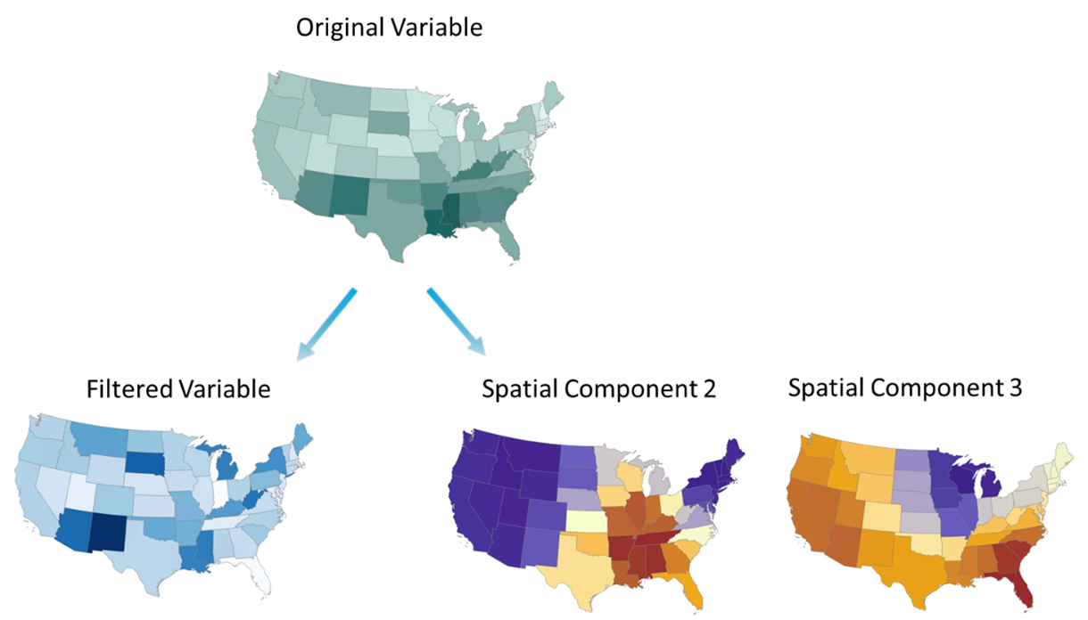
This tool becomes very useful in two scenarios. First, it helps us to explore the relationship between two variables while reducing the interference of neighboring influences. Second, it enhances regression and machine learning models by eliminating spatial misspecifications and can make non-spatial models become spatial models. The rest of this blog article will show examples of these two scenarios.

Data used in this article

• Boston Housing data: a famous benchmark dataset from http://lib.stat.cmu.edu/datasets/boston.
• County-level census data in Ohio by ArcGIS Pro Enrich tool.

Application 1: Is it correlation or is it Tobler’s First Law?

“How is a researcher to know if variable y and variable x are related to each other in a meaningful way, or if they only appear to be related because “everything is related to everything else?” (Thayn, 2017)

As a geographer or a GIS analyst, we recognize that most phenomena do not exist independently from space. We believe Tobler’s first law of geography – “everything is related to everything else, but near things are more related than distant things.” This unique aspect of spatial data often violates the statistical assumption that observations are independent of each other. As such, when assessing the relationship between two variables, discerning whether their relationship is genuine or merely a result of significant spatial autocorrelation becomes difficult.

For instance, Fig 2 is a scatter plot showing the relationship between the proportion of old houses and the concentration of nitric oxide in Boston. This chart suggests that there is a positive relationship. As the proportion of older houses increases, the concentration of nitric oxide also rises.

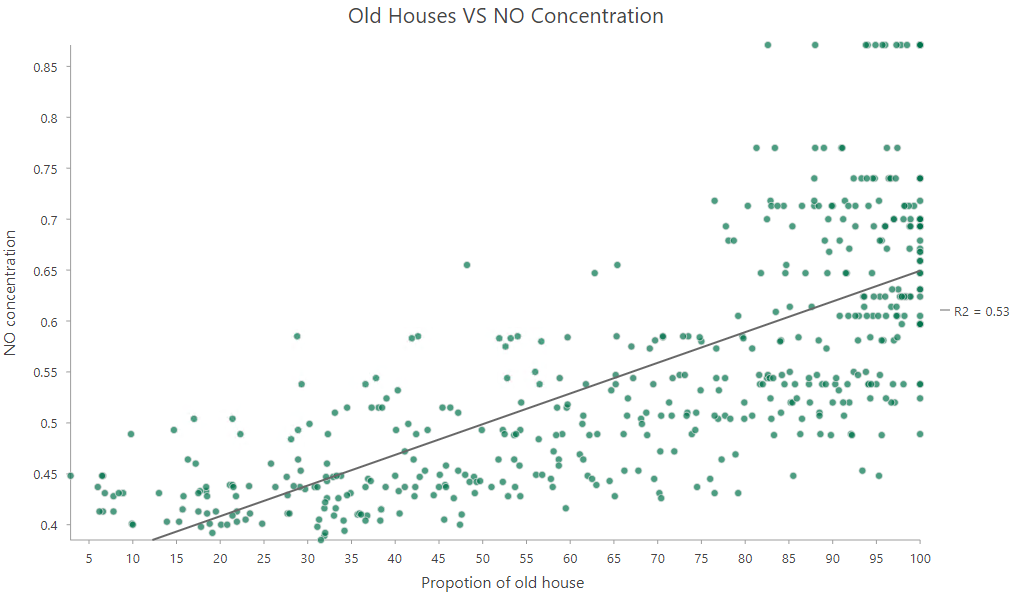
However, when observations are influenced by their neighboring data points, determining the strong positive relationship depicted in Fig 2 becomes challenging, as this could be due to the confounding impact of the spatial autocorrelation. If you look at the maps of Old Houses and NO (Fig 3 and Fig 4), you will notice that both variables exhibit strong spatial clustering.

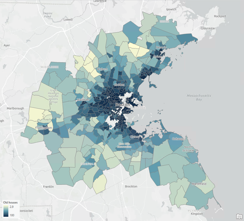
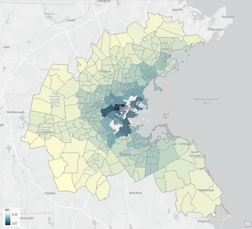
This is where the Filter Spatial Autocorrelation From Filed tool comes into play. It helps us to isolate the spatial component from a variable, allowing us to investigate the relationship between two variables independently of the influence of their neighbors. In the tool, I first select the Boston data as the Input Features. Then later, Fig 5 and Fig 6 show the tool dialog used to filter the house age and nitric oxide fields.

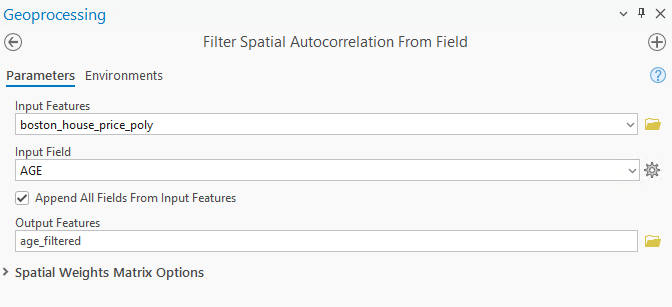
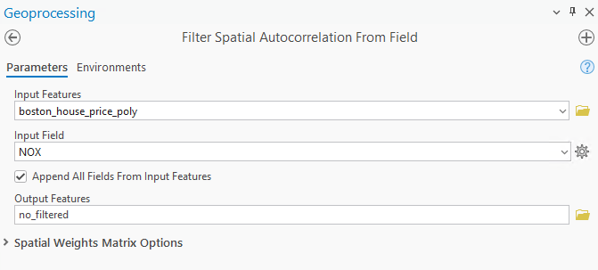
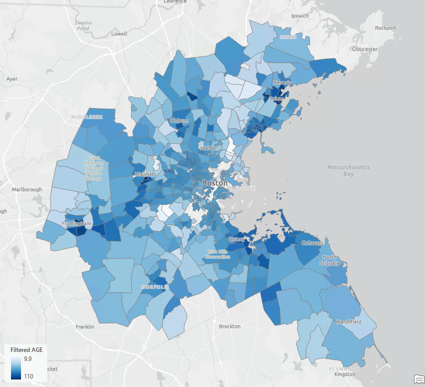
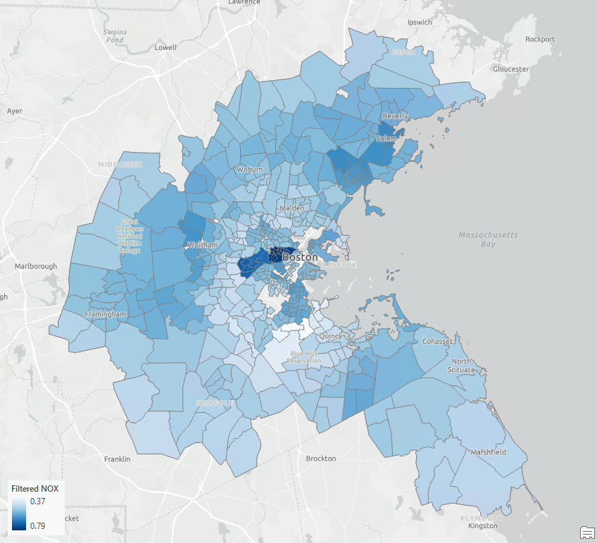
I have generated two outputs by running this tool twice. One output map is symbolized based on the Filtered AGE, representing the proportion of old houses in Boston without the spatial influence (see Fig 7). The second map illustrates the Filtered Nitric Oxide, showing the concentration of NO after filtering the spatial autocorrelation (refer to Fig 8).

The filtering steps can be found in the geoprocessing messages. For example, Fig 9 demonstrates how the spatial autocorrelation present in AGE is removed after four iterations. Initially, the Moran’s I index is 0.3206 with a P-value of 0.001, indicating a significant spatial autocorrelation. After filtering four spatial components from AGE, Moran’s I index decreases, and the P-value increases to 0.99. This change tells us that the spatial autocorrelation is no longer significant.

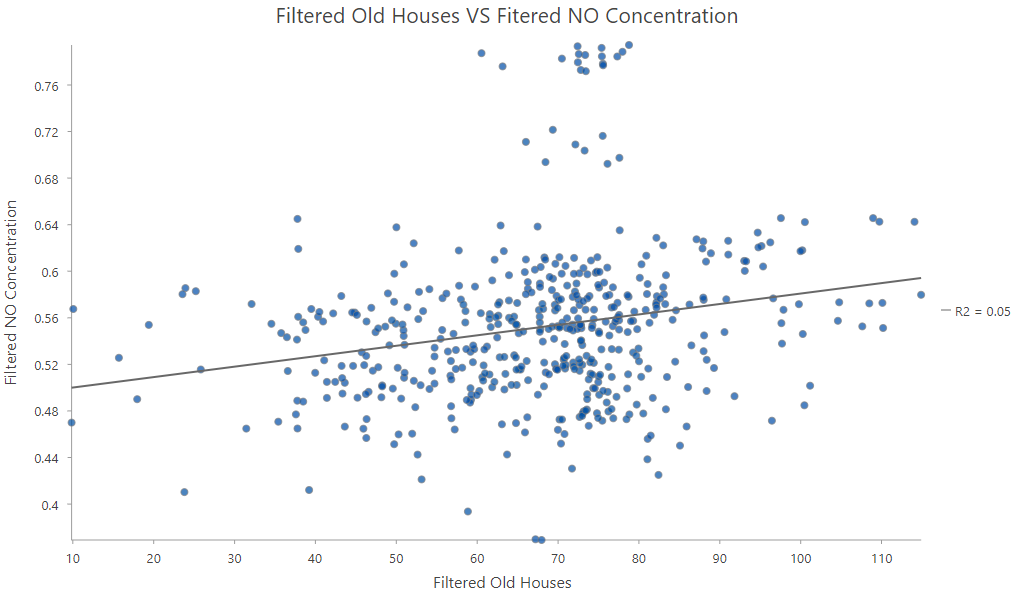
Now, Fig 10 shows the relationship between the two variables after filtering out the impact of space. Comparing Fig 2 with Fig 10, we will find that the strong positive relationship shown in Fig 2 is largely due to shared spatial relationships, but some correlation still remains after filtering out the spatial relationships.

Application 2: Bring space into non-spatial models

As mentioned previously, spatial data often violates the assumption of traditional statistical methods which leads to biased estimates and questionable results. However, by integrating the spatial components returned from the Filter Spatial Autocorrelation From Field tool, we can incorporate the spatial information into a non-spatial model, transforming it into a spatially-aware model.

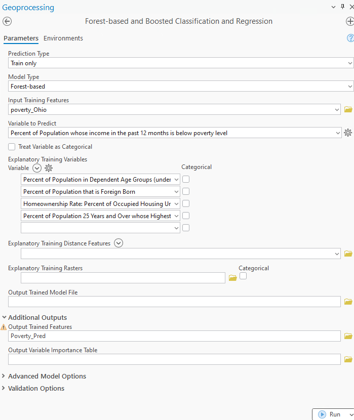
Here is one example. I have demographic data from Ohio, and I used the Forest-based and Boosted Classification and Regression tool to construct a forest-based model.  My goal is to gain a deeper understanding of poverty factors and estimate the poverty percentage after implementing potential intervention plans.

I selected Percent of Population whose income in the past 12 months is below poverty level as the Input Variable to Predict. The Explanatory Training Variables chosen include:

1. Percent of Population in Dependent Age Groups (under 18 and 65+)
2. Percent of Population that is Foreign Born
3. Homeownership Rate: Percent of Occupied Housing Units that are Owner-Occupied
4. Percent of Population 25 Years and Over whose Highest Education Completed is Bachelor’s Degree or Higher.

Finally, I saved the Output Trained Features as Poverty_Pred, and hit Run (refer to Fig. 11).

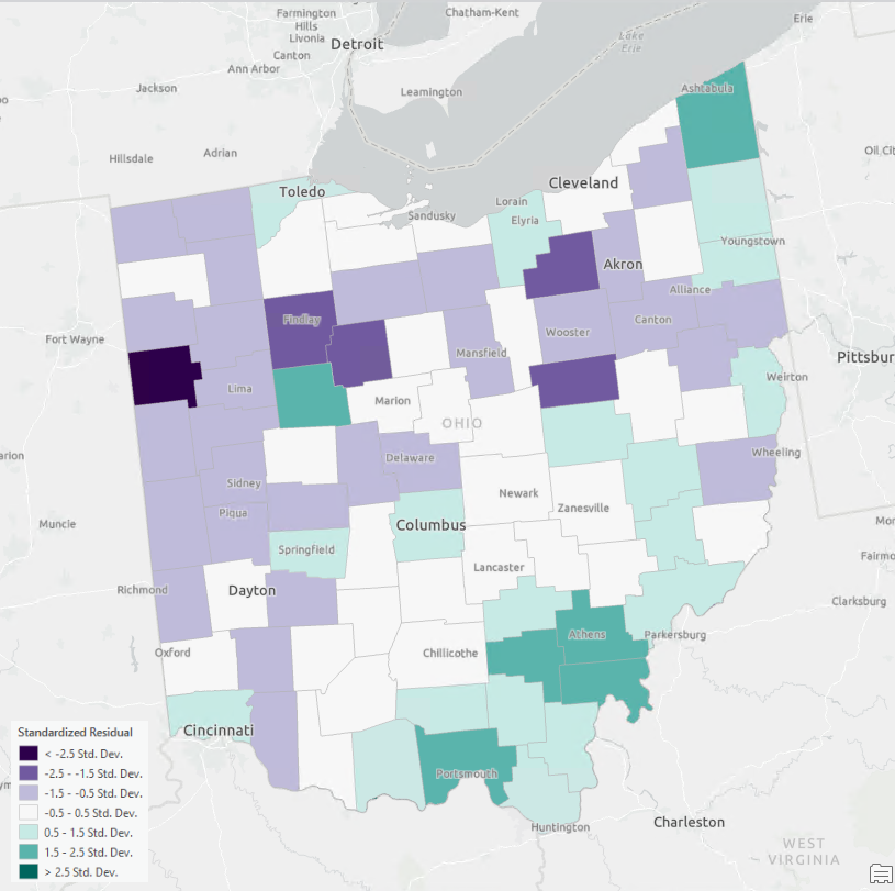
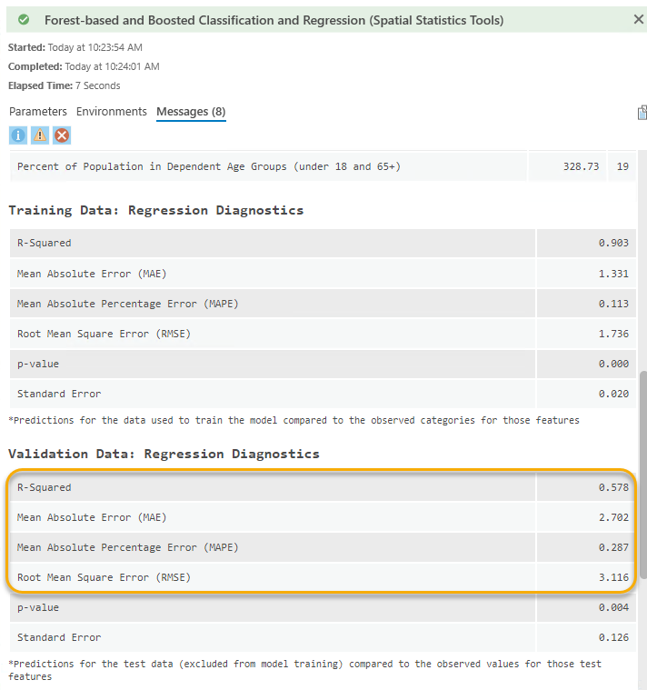
After running the tool, I got an output trained layer displaying its standardized residuals (Fig 12). Let’s look at the map, and two clusters can be noticed: counties shaded in green are situated in the Southeast, while those in purple are clustered in the Northwest. This residual map suggests that the model tends to underestimate the poverty (%) in the Southeast region while overestimating it in the Northwest region. In other words, there is notable spatial autocorrelation present in the model’s residuals.  This highlights unequal predictive power across regions, indicating that this forest-based model fails to explain a certain spatial pattern present in the data. The model performance also needs to be improved as the validation R-squared is 0.578 currently (Fig 13).

To tackle the spatial bias n my forest-based model, I used the Filter Spatial Autocorrelation From Field tool.

1. I opened the tool, and selected Poverty_Pred, the output generated from my forest-based model, as the Input Features.
2. I selected Standardized Residual as the Input Field, specified Poverty_Pred_FilterSpatialAutocorrelationFromField as the Output Features, and
3. ran the tool (Fig 14).

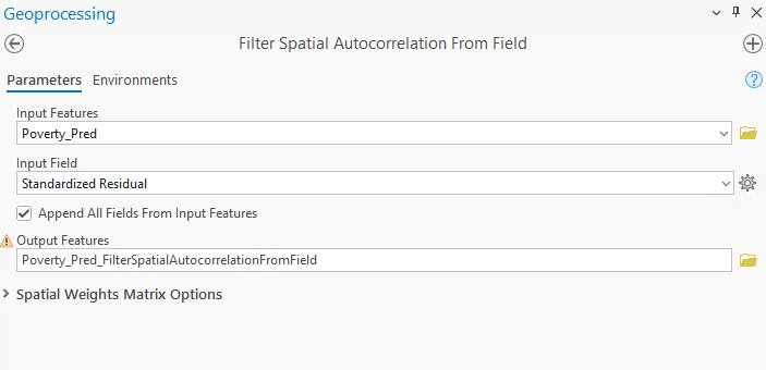
The Output Features generated from this tool not only contain the filtered input field but also the spatial components isolated from the input field. In this case, the spatial components represent the spatial pattern that cannot be explained by the forest-based model we saw in Fig 12. Therefore, after including this spatial component in my forest-based model, the model may be able to address the unequal spatial distribution of predictive power.

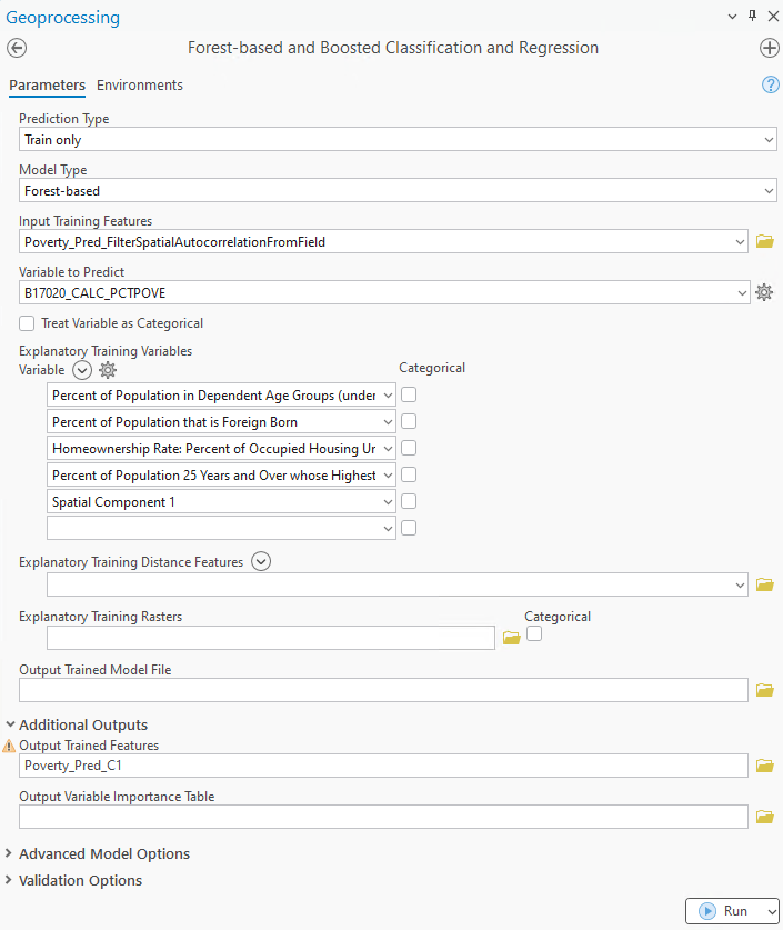
1. I re-opened the Forest-based and Boosted Classification and Regression Instead of the original poverty_Ohio,
2. I selected the Poverty_Pred_FilterSpatialAutocorrelationFromField as the Input Training Features.
3. I kept most of the Variable to Predict and Explanatory Training Variables consistent with Fig. 11, while adding the spatial component as an additional explanatory training variables.
4. Then, hit ran. (see Fig 15)

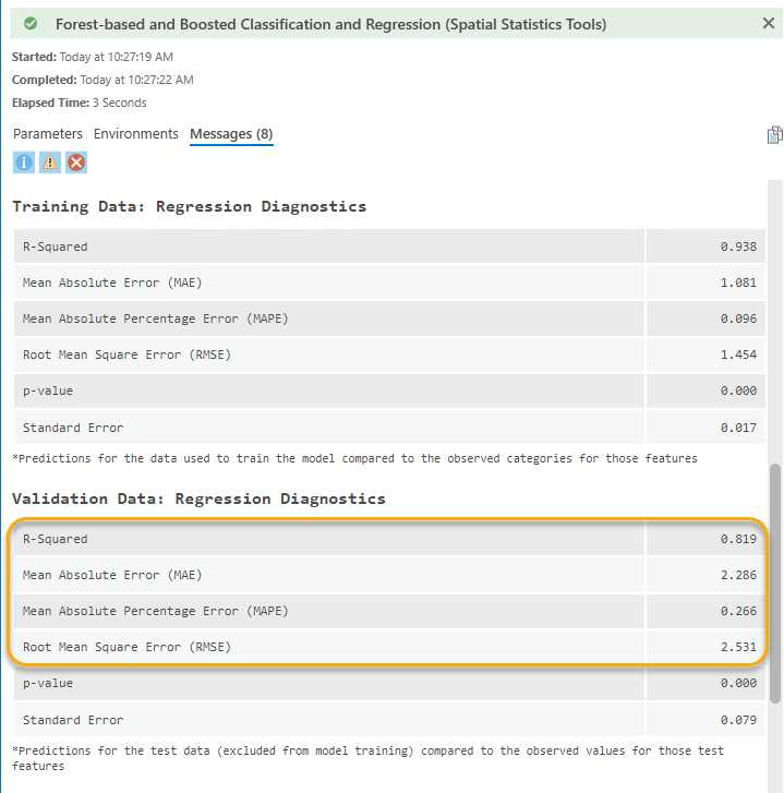
The effectiveness of this improvement is shown in Fig 16. The training R-squared as increased from 0.903 to 0.938. More importantly, the validation R2 saw a notable increase from 0.578 to 0.819, accompanied by reductions in all errors, including MAE, MAPE, and RMSE. This improved forest-based model indicates that the model is more reliable, and we are more confident in interpreting the variable importance and estimating the poverty percentage.

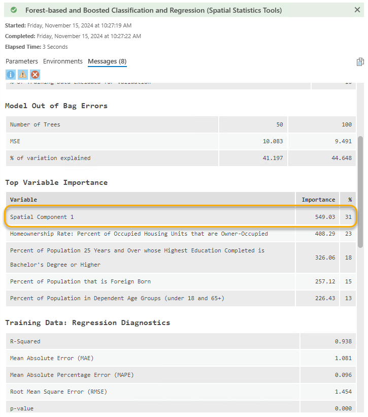
Let’s look at the variable importance (Fig 17), and we will notice the spatial component I added into the model is on the top. The spatial component is capturing a spatial process that we do not have in our original training dataset that may be a key indicator of poverty in Ohio.

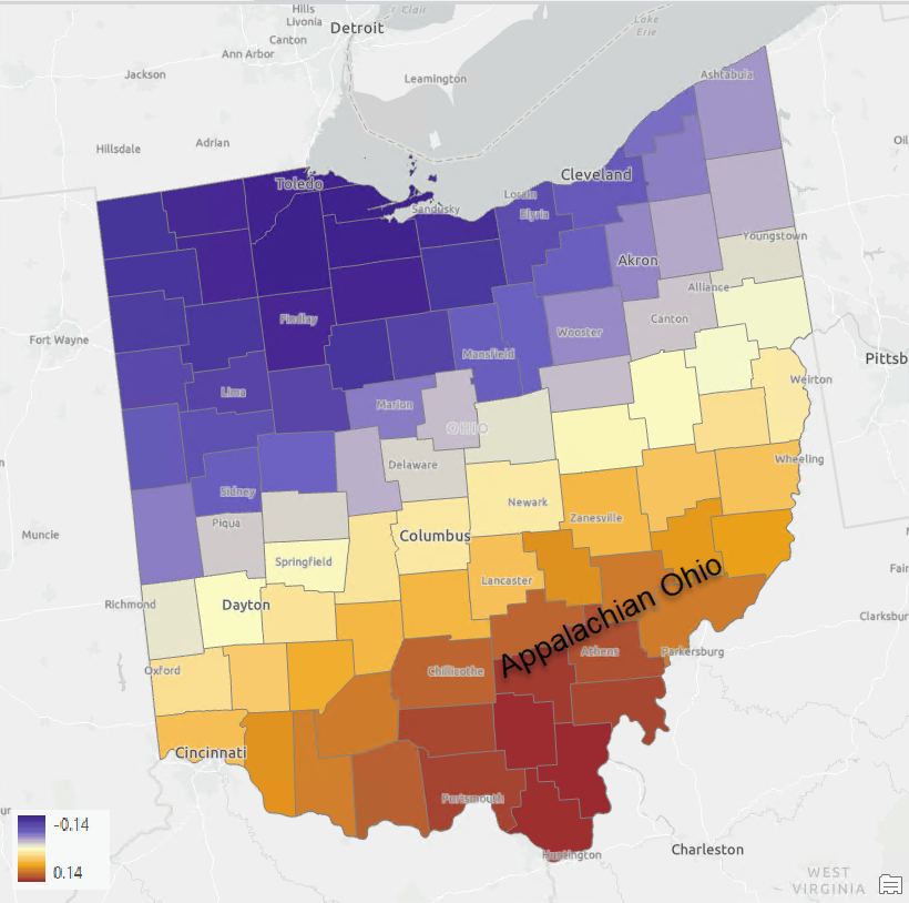
I can even map the spatial component to see the spatial pattern that greatly impacts the poverty percentage (as shown in Fig 18). The pattern of this component showing higher values in the Appalachian Ohio region and lower values in the Non-Appalachian Ohio region suggests that we should focus on this distinct spatial difference when trying to mitigate poverty in Ohio. The spatial component also provides us the insights into what real-world variables we should incorporate into the model. The spatial components should be used as a stand-in when we do not know which variables we may be missing. Whenever possible, a measured alternative is always recommended.

Conclusion

In this blog article, we showcase how the Filter Spatial Autocorrelation From Field tool can be beneficial in two scenarios. First, it helps us evaluate the relationship between two variables by filtering out the impact of space. Secondly, the spatial components can serve as proxy variables for important explanatory variables missing from the model. By adding the components into a non-spatial machine learning model, the model is turned into a spatial model without modifying the structure of the model. Additionally, the spatial components isolated from the residuals provide valuable insights into the real-world variables that may have been overlooked in our model. As this tool is so powerful, I am eager to see how this tool will help your spatial data analysis!

Thayn, Jonathan B. “Eigenvector Spatial Filtering and Spatial Autoregression.” (2017): 511-522.