The Spatial Analyst team has made some important improvements in the Distance toolset for ArcGIS Pro 2.5.
We have significantly improved the precision of the geoprocessing tools in the Distance toolset and the corresponding raster functions. We have also provided additional capabilities which let you answer some new “how much/how many/how far” questions.
These improvements allows us to remove the strong distinction between the “Euclidean” and “Cost” Distance tools. The number of tools has been reduced from 17 to 6. The new user experience is now simplified to:
- Enter Sources
- Do you have barriers?
- Do you have a surface?
- Do you have a cost surface?
- Do you need to consider direction of motion and other source characteristics?
The new toolset organization is shown in Figure 1 below. The new tools are:
- Distance Accumulation
- Distance Allocation
- Optimal Path As Line
- Optimal Path As Raster
- Optimal Region Connections
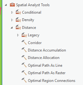
The original Distance tools that you are familiar with are available in the Legacy sub-toolset.
The Spatial Analyst team recommends that you move your Euclidean and Cost Distance analysis work to the new tools.
Why should I use the new tools?
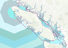
At ArcGIS Pro 2.5, we’ve uniformly adopted a new algorithm [4] for all distance mapping tools. This algorithm removes the distortion in outputs caused by using a network model of cell connectivity, as shown in Figure 2 on the left below. This has the following benefits:
- Cost distance is now measured the same way in all directions. An important special case is cost distance with a constant cost surface now produces the same output as the Euclidean distance tools.
- Surface distance over a digital elevation model can now be precisely computed.
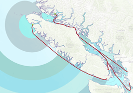
- Paths around barriers are now followed precisely, as shown in Figure 3.
 |
 |
At ArcGIS Pro 2.4, we introduced this improvement in a limited context: Euclidean distance with barriers. ArcGIS Pro 2.5 generalizes and extends this work.
What else is new?
Along with this fundamental change to the behavior of the cost distance algorithm, several additional capabilities have been added.
- You can use geodesic distance with the Distance Accumulation, Distance Allocation, and Optimal Region Connections tools.
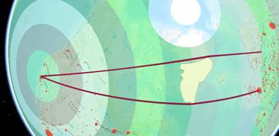
Figure 4- Geodesic flight paths from some Northern European airports to LAX, but avoiding paths over southern Greenland. - As a side effect of the improved algorithm, you can now create buffer regions whose distance is measured over the surface of a digital elevation model. This isn’t really a separate capability, but it’s important enough to mention explicitly. In the example below, the study area is Lake Wakatipu near Queenstown, New Zealand – a high relief area. Notice how, in such areas, the output of the Distance Accumulation tool (gray gradient) with a maximum accumulation cutoff of 1500m “pulls away” from the output of the vector Buffer tool that used a buffer distance of 1500m. This surface-aware distance computation can be done in either planar or geodesic mode.
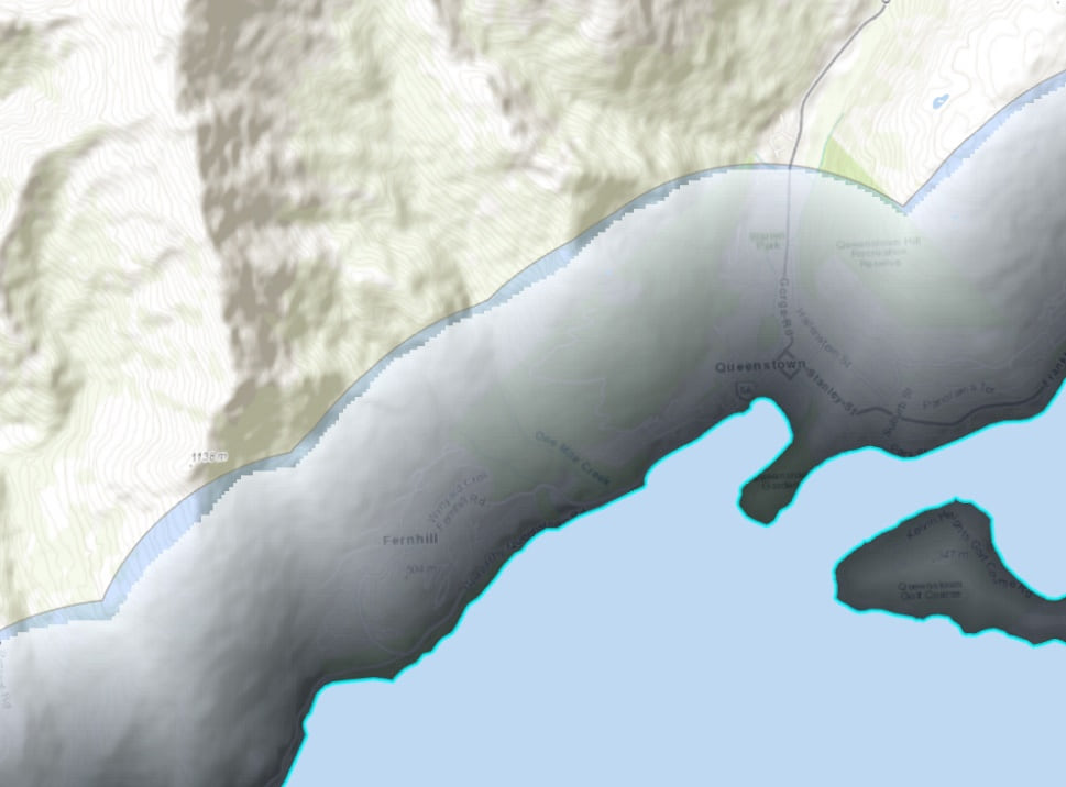
Figure 5 – Comparison of planar (blue) and surface distance (gray gradient) buffers around Lake Wakatipu in the Queenstown area of New Zealand. Both buffers extend to a distance of 1500m, but the gray gradient output measures distance over the surface of a DEM instead of distance in the plane of the data’s projected coordinate system. - Using the new Optimal Path as Raster tool, you can count how many least cost paths pass through a cell en route from some destinations to a source.

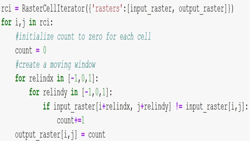
Figure 6 – Optimal Path As Raster output from ridgeline hiking trail in SW to access road in NE. Green is less intense usage, red is more intense. - Using the new source_location output from Distance Accumulation and Distance Allocation, you can do intensity mapping of the boundary of sources, showing where most cost paths in the study area would end up, without plotting all cost paths. The RasterCellIterator python object, also new at ArcGIS Pro 2.5, makes this type of intensity calculation very easy to perform. See A quick tour of using Raster Cell Iterator to know more about it.
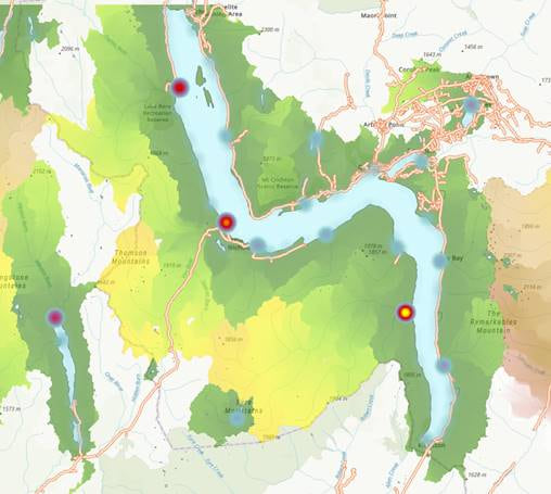
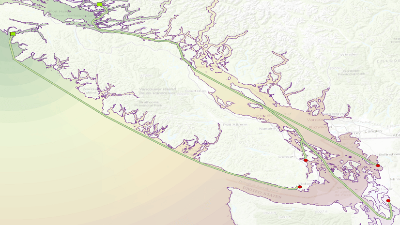
Figure 7 – Lake Wakatipu, New Zealand. Hot spots (red and blue fuzzy dots), computed from Distance Accumulation output, show locations of most intense drainage into lake from surrounding watershed.
Which geoprocessing tools and raster functions should I start using?
For each legacy distance tool that you are currently using, table 1 shows you which new tool to switch to.
| If you used | Then switch to |
|---|---|
| Cost Distance | Distance Accumulation |
| Cost Backlink | Distance Accumulation with back direction output |
| Cost Allocation | Distance Allocation |
| Euclidean Distance | Distance Accumulation |
| Euclidean Allocation | Distance Allocation |
| Euclidean Direction | Distance Accumulation with source direction output |
| Path Distance | Distance Accumulation |
| Path Backlink | Distance Accumulation with back direction output |
| Path Allocation | Distance Allocation |
| Cost Path | Optimal Path As Raster |
| Cost Path As Polyline | Optimal Path As Line |
| Cost Connectivity | Optimal Region Connections |
For new workflows, the back direction raster replaces the back link raster. The Optimal Path as Raster/Line tools no longer accept a backlink raster as input (they will still accept a flow direction raster). If you were using the backlink raster in a workflow that involves something other than the Cost Path or Cost Path As Polyline tools, then the Spatial Analyst team would like to hear from you. The Euclidean distance blog mentioned above discusses the backdirection raster in more detail.
If you used the maximum_distance parameter in the legacy cost tools, you should now use the Maximum Accumulation parameter in the “Characteristics of the sources” parameter group.
These are the new raster functions.
The functions have the same parameters as the tools, with an important difference: the functions optionally emit multi-band outputs. This avoids having to run these (possibly expensive) global functions twice to get closely related outputs (like accumulated cost surface and back direction raster).
Also, the Least Cost Path raster function has been updated to use the Distance Accumulation tool behind the scenes.
Finally, although not directly related to these enhancements, your advanced use of the Distance toolset needs to consider if direction of motion between sources and destinations is important. If so, please check out this blog on Creating accumulative cost surfaces using directional data.
References
1) Goodchild, M. F. (1977). An Evaluation of Lattice Solutions to the Problem of Corridor Location. Environment and Planning A. 9. 727-738. 10.1068/a090727.
2) Sethian, J. A. (1997). Tracking Interfaces with Level Sets: An “act of violence” helps solve evolving interface problems in geometry, fluid mechanics, robotic navigation and materials sciences. American Scientist Vol. 85, No. 3 (MAY-JUNE 1997), pp. 254-263
3) Sethian, J. A. (1999). Level set methods and fast marching methods: evolving interfaces in computational geometry, fluid mechanics, computer vision, and materials science (2nd edition). Cambridge University Press.
4) Zhao, H. (2005). A fast sweeping method for eikonal equations. Mathematics of computation, 74(250), 603-627.
Commenting is not enabled for this article.