***Please note that all Telecom Domain examples are Beta 2
During IMGIS 2025, we had the opportunity to present the new Telecom Domain as a part of the plenary presentation for the ArcGIS Utility Network. Currently it is still a beta release but there are a number of new features we were excited to demonstrate. This blog is intended to provide a little more detail specific to the new features and framework.
The first production release of the Telecom Domain within the ArcGIS Utility Network will be included in the spring 2026 Network Management (ArcGIS Pro 3.7 and ArcGIS Enterprise 12.1) release. Using this new data structure, we can model our fiber system at a new level of detail. This includes representation of our network all the way down to the fiber strand or port level. Examining the graphic below (Image 1) we can see how a fiber cable is complex with strands in bundles of tubes.

To model those strands, we can use three of the new capabilities- grouping, circuit management, and tracing.
Let’s get into grouping first where we can reduce the number of relationships we manage.
Grouping —
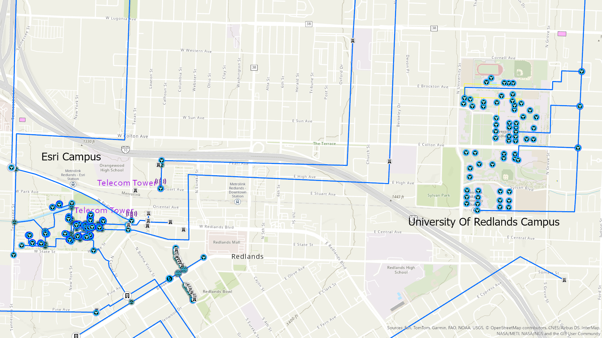
Grouping is helpful when tracking fibers in a cable or ports in a device. The graphic below represents a sample utility network extending from the Esri headquarters to the University of Redlands campus. In the graphic below (Image 2), we select the cable that represents the backbone between the two campuses. We can see the fiber inside of this cable, including the first and last strand unit numbers. Highlighting the last unit value tells us we have 96 strands of fiber inside the cable. Diving deeper, we can see the connected ports and corresponding unit values for the ports; one for each fiber strand. In this case, grouping allowed us to reduce 96 nonspatial fiber records and 96 containment cable associations to just one record and one association. Grouping ultimately gives us the ability to manage more complex networks with greater efficiency.
Circuit Management —
Circuit management allows us to accurately reflect fiber maintenance activities. By logically portraying areas of connectivity within a fiber network, we can mirror configurations commonly seen with telecom systems. In this new domain, all telecom circuit management is location-based and a function of identifying start and stop locations at the circuit or section level. With the new circuit tools, we can model our network by location, break it into sub-circuits (where circuits share elements with each other) or sections, and manage it as complete logical paths with no controllers for better alignment with real-world telecom networks. To better understand how circuits are managed, we can use the Find Circuit toolbox. This new toolbox offers a one-click experience with access to popular tools and functionality, such as trace, modify, export, and validate, making them easier to access and utilize efficiently.
As an example of the new circuit management capabilities, let’s explore a circuit that represents the backbone connection between the Esri Internet Service Provider (ISP) and the northern tap off of the University campus. Leveraging the Modify Circuit tool (see Image 3 below), we can explore the details of this circuit’s location.

Tracing —
Tracing allows users to select paths through the network starting from one or more points (such as devices, junctions, or subnetwork controllers) and expanding outward until reaching barriers, endpoints, or defined conditions. Because of the grouping capability, tracing is enhanced to enable richer visualization of our telecom data. Using the Find Circuits tool we can now execute telecom focused traces with only one click (Image 4).
We have identified a bunch of cable running through the University of Redlands campus (Image 5). We are using this cable to select only the attributes for the bundle inside. Although the cable selection has now cleared on our map, we know our fiber is still selected because it is the remaining attribute listed. We established a starting point for our trace by loading the selected fiber into the trace window. The first strand is displayed by default. Using the dropdowns, we can execute a trace on any or all strands within this selection. This is important news for utility network users because now we can trace any nonspatial features grouped within an individual fiber or port.
Using the utility network tool gallery, we will chose the connected trace option. Opening the geoprocessing tool, we check the boxes for containers and content to ensure spatial and nonspatial features are included in our results. Running the trace returns the path for strand 1 in our cable, visualizing it along with its devices.
We can easily rerun our trace along multiple strands in this cable by changing the unit values (Image 6). All of the strands we set in our value range are now shown in the map.
The color abbreviation next to the strand numbers is also important. These colors are configurable within the domain properties to match existing network equipment relating to individual strands in a bundle and to bundles in a cable (Image 7). This helps field crews do their jobs more efficiently, allowing them to quickly identify fiber properties.
Finally, we can execute traces across disconnected service areas, as well as infer connectivity across devices (Image 8). This is the case with these towers. Analyzing all network assets helps provide an interface that is more reflective of a telecom system and streamlines the experience for users.
Right now the Telecom Domain is a beta product and will be released into production with the Network Management release of 2026. This new domain is neither a replacement for the existing Communications Foundation data model nor does it substitute existing utility networks developed under traditional communications domain infrastructure. Instead it is simply an alternative to help customers model their fiber systems.
The Telecom Domain empowers communications infrastructure across all industries to fully embrace the revolutionary visualization and analytic tools that come with an ArcGIS Utility Network. We will have a few follow-up blogs to discuss capabilities of beta-2 and more details as we get closer to the release coming this spring.


Commenting is not enabled for this article.