Deep learning models trained on ImageNet have long been the default choice as backbones for various computer vision tasks. However, when applied to geospatial problems, they often struggle due to the fundamental differences between natural images and remote sensing imagery. In recent years, the advent of foundation models has revolutionized the field of artificial intelligence. These models, trained on extensive datasets, have demonstrated remarkable versatility across a wide array of tasks. In the realm of remote sensing, specialized foundation models like IBM and NASA’s and the Dynamic One-For-All (DOFA) model have emerged, offering significant advantages over traditional backbones trained on ImageNet.
My previous blog article explored how self-supervised geospatial backbone models outperform traditional Imagenet-pretrained counterparts on downstream geospatial tasks owing to their domain specific feature representations. This blog article explores why remote sensing foundation models, which are trained on large scale data, serve as better backbones for geospatial deep learning and how they can be leveraged within the ArcGIS ecosystem.
Foundation models
At a high level, foundation models are large deep learning models trained on large, diverse datasets to perform a range of tasks. By learning from diverse and extensive data, these models capture a variety of features and patterns, enabling them to be effectively adapted (fine-tuned) for downstream tasks with relatively less task-specific data. Instead of training a new model from scratch for each problem, you can start with a strong foundation and build upon it.

Essential building blocks of foundation models
Foundation models, especially in recent advancements, rely on a few key elements:
- The transformer architecture with attention mechanism—Architecture that has impacted various fields, including natural language processing and computer vision. At its core lies the attention mechanism, which allows the model to weigh the importance of parts of the input data when making predictions. This enables the model to capture long-range dependencies and understand the context within the data more effectively than traditional convolutional networks alone. Architectures like Vision Transformers (ViTs) are prime examples of this when applied to computer vision.
- Large-scale data—Foundation models are trained on massive and diverse datasets. For remote sensing, this means ingesting terabytes of satellite imagery, aerial photos, and other geospatial data from various sensors and covering different geographical locations and time periods. This vast amount of data allows the model to learn generalizable features applicable to a wide range of scenarios.
- Large compute—Training these massive models on such extensive datasets requires significant computational resources. This often involves using powerful clusters of GPUs or TPUs for extended periods. The sheer scale of computation enables the model to learn complex patterns and representations from the data.
These three elements are fundamental to the development and success of modern foundation models.
Remote sensing foundation models
Recent advancements in geospatial AI have led to the development of foundation models pretrained on large-scale geospatial datasets. These models learn domain-specific representations and significantly outperform traditional backbones in geospatial tasks.
Prithvi (IBM and NASA’s model)

The Prithvi-EO-1.0 model, a collaborative effort between IBM and NASA, is a significant step forward in remote sensing foundation models. Trained on a massive dataset of Harmonized Landsat and Sentinel-2 (HLS) imagery, Prithvi has demonstrated impressive capabilities across various downstream tasks, including land cover mapping, flood detection, and more.
Its architecture is based on a self-supervised encoder using a Vision Transformer (ViT) backbone, enhanced with a Masked Auto Encoder (MAE) learning strategy. An asymmetric decoder with a Mean Squared Error (MSE) loss function reconstructs the masked images, thereby learning in a self-supervised manner. To effectively handle spatiotemporal data, the model incorporates 3D patch embeddings and 3D positional embeddings, replacing traditional 2D counterparts. These 3D embeddings allow the model to capture spatial and temporal relationships within the data more effectively.
Additionally, Prithvi-EO-1.0 integrates infrared bands alongside standard RGB channels, specifically using six spectral bands from NASA’s Harmonized Landsat and Sentinel-2 (HLS) data: Blue, Green, Red, Narrow NIR, SWIR 1, and SWIR 2. These architectural enhancements enable Prithvi-EO-1.0 to perform comprehensive analyses of Earth’s surface changes over time. Its pretraining on a globally consistent and temporally rich dataset allows it to learn robust representations that are transferable to diverse geographical locations and environmental conditions.
The Prithvi model has also been fine-tuned for Burn Scar segmentation, Flood Segmentation, and Crop Classification by IBM and NASA. These task specific variants are available in ArcGIS Living Atlas as pretrained deep learning packages.

Learn more in the reference paper Foundation Models for Generalist Geospatial Artificial Intelligence
Dynamic One for All (DOFA) model

The Dynamic One-For-All (DOFA) model is a multimodal foundation model tailored for remote sensing and Earth observation tasks. Inspired by neural plasticity—the brain’s capacity to adapt to new experiences—DOFA is designed to process diverse data modalities within a unified framework, thereby enhancing its versatility across various Earth observation applications.
DOFA builds on the principles of masked image modelling, introducing a significant advancement by processing input images with any number of channels. This is enabled by a hypernetwork-based dynamic weight generator, which adapts to the spectral wavelength of each channel. By embedding images with varying channel numbers into a unified feature space, the model leverages shared transformer networks to learn modality-shared representations. This architecture enables the model to learn versatile multimodal representations and handle diverse data modalities within a single framework.

In summary, DOFA consists of four parts: 1) wavelength-conditioned dynamic patch embedding; 2) multimodal pretraining with shared transformer networks; 3) masked image modelling with a variable number of spectral bands; and 4) distillation-based multimodal continual pretraining.
Learn more in the reference paper Neural Plasticity-Inspired Multimodal Foundation Model for Earth Observation
How remote sensing foundation models differ from ImageNet backbones
As highlighted in the previous blog post, while ImageNet pretraining has been a valuable starting point, it suffers from a domain gap. Natural images and remote sensing imagery have fundamentally different characteristics in terms of spectral information, spatial resolution, and the types of objects and phenomena they capture.
Remote sensing foundation models, trained on massive datasets of satellite and aerial imagery, learn features that are inherently relevant to Earth observation tasks. This leads to the following:
- Improved performance—They often achieve higher accuracy and better generalization on downstream remote sensing tasks compared to ImageNet-pretrained backbones.
- Faster convergence—They require less task-specific data and fewer training epochs to reach a desired level of performance.
- Better feature extraction—They capture spectral signatures, spatial relationships, and contextual information specific to geospatial data.
 is reported, and the best results are shown in bold. Source: Xiong et al.")
Use these backbones in ArcGIS
You can use these remote sensing foundation models to train your task-specific models using ArcGIS. The Deep Learning Tools in ArcGIS Pro’s Image Analyst toolbox allow you to use these models as backbones without coding.
The models can also be trained on data with any number of bands and, in the case of DOFA, on imagery from multiple sensors.
Adapt remote sensing models as backbones
Models like Prithvi and DOFA are built upon the popular Vision Transformer (ViT) architecture. Unlike conventional convolutional networks, Vision Transformers (ViTs) use a plain, nonhierarchical architecture that maintains a single-scale feature map throughout. This design poses challenges for tasks like object detection, where the key question arises: How can multiscale objects within an image be effectively detected? Additionally, downstream tasks such as object detection and segmentation typically benefit from high-resolution images. However, architectures like ViT become computationally expensive and inefficient at such scales due to the quadratic complexity of the self-attention mechanism.
To address these challenges, inspiration was taken from Meta AI’s popular ViTDet and these remote sensing foundation models were adapted as effective pretrained backbones with minimal modifications. Specifically, a simple feature pyramid is constructed using only the final feature map from these ViT-based models. Specifically, with the default ViT ’s last feature map of scale 1/16 (stride = 16), feature maps of scales { 1/32 , 1/16 , 1/8 , 1/4 } are produced using convolutions of strides {2, 1, 1/2 , 1/4 }, where a fractional stride indicates a deconvolution.
This approach eliminates the need for significant alterations to the original backbone, unlike hierarchical designs such as Swin Transformers, while allowing the model to detect features at multiple scales. To enable efficient feature extraction from high-resolution images while reducing computational overhead, a nonoverlapping window attention mechanism (without shifting) was introduced. A small number of global attention blocks are employed to facilitate information propagation. Importantly, these adaptations are applied only during fine-tuning and do not modify the pretrained weights. The graphic below shows the architectural modifications done to adapt remote sensing models into effective backbones.

Export training data
You’ll start by exporting training data for the task at hand. The Export Training Data for Deep Learning tool with the Classified Tiles metadata format is used to export training data for the model in this example.
Refer to the Land cover classification using sparse training data sample notebook for more details on data export for pixel classification tasks.
Fine-tuning the Prithvi backbone using ArcGIS Pro
Once you have the exported data ready in a folder, you can train Pixel Classification models on this data. In the example workflow below, you will finetune a Deeplabv3 model with Prithvi model as a backbone on an exported pixel classification dataset.
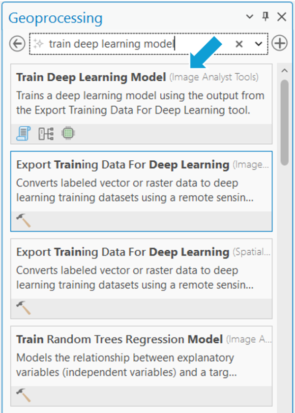
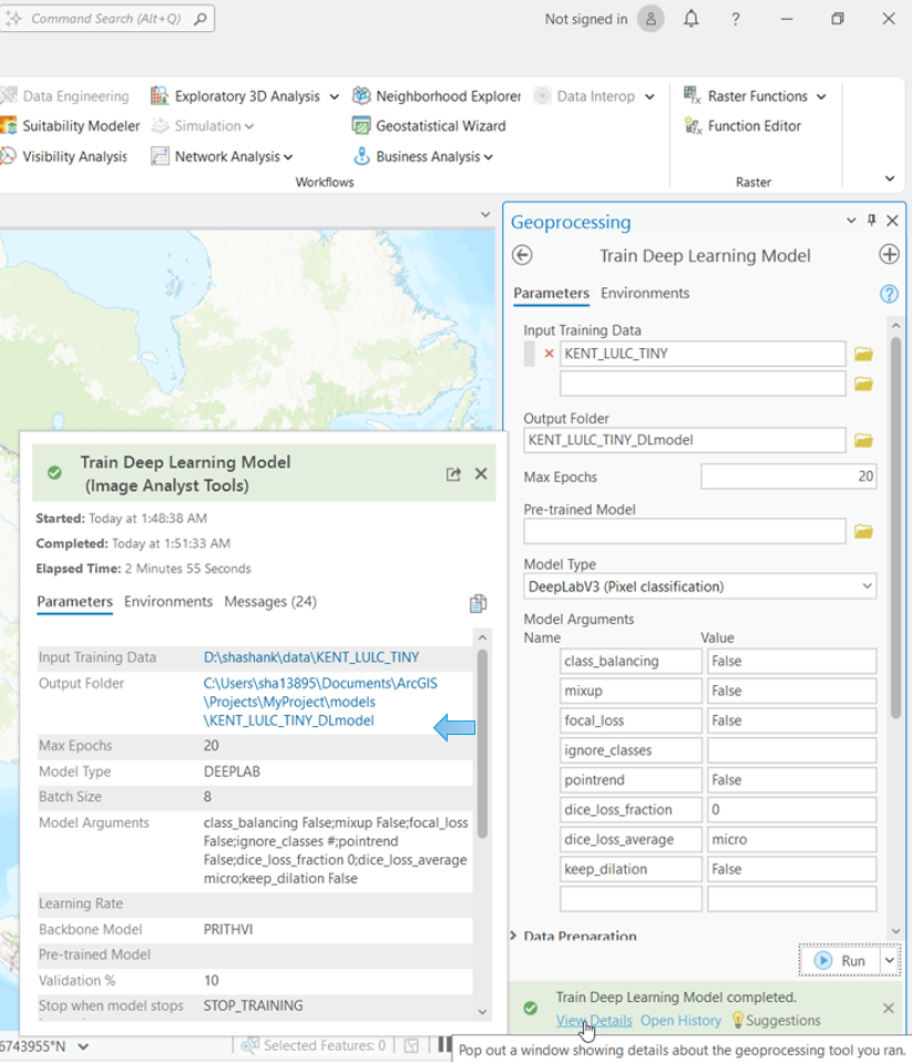
- On the Analysis tab, click Tools > Geoprocessing > Search and open Train Deep Learning Model.
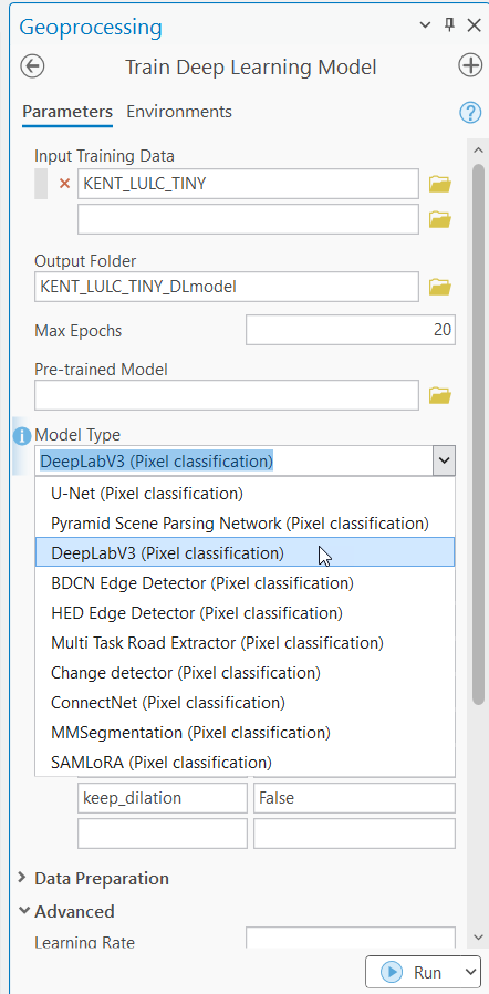
- Enter the path of the exported data in the Input Training Data
- If you want to resume the training from an existing checkpoint, enter the path of the model in the Pre-trained Model
- Select DeepLabv3 (Pixel classification) from the Model Type drop-down menu.
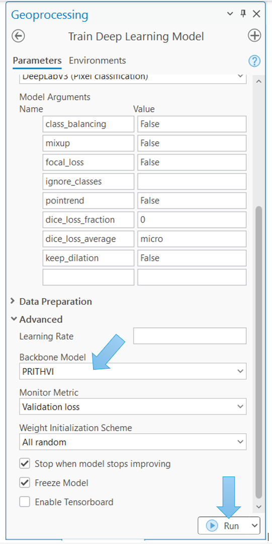
- To select Prithvi as a backbone, expand the Advanced section and in the Backbone Model field, select the PRITHVI model from the drop-down menu.
- Optionally, keep the default values for the rest of the fields or modify them accordingly.
- Click Run to start the model training.
The tool starts the model training.
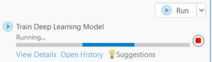
Upon completion, the model will be saved in the Output Folder location as a deep learning package, which can then be used for inference.
Fine-tune the DOFA backbone using ArcGIS API for Python
These foundation models have been integrated as backbones in the arcgis.learn module of ArcGIS API for Python for a low-code experience.
The following is the same example of training a Deeplabv3 model with DOFA backbone on the exported Pixel classification dataset (Land cover classification), but this example uses arcgis.learn.
Required imports
from arcgis.learn import prepare_data, DeepLab
Prepare training data
Pass the path of the exported data as an argument into the prepare_data function:
data = prepare_data(path, batch_size=4, chip_size=256)
Visualize training samples
data.show_batch()
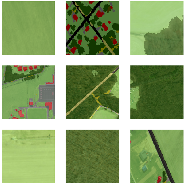
The labels are overlaid on the original image with transparency, each unique color representing a unique class.
Initialize the DeepLab model
The following example uses a dofa_base backbone. You’ll use the backbone argument in the constructor to specify the same.
model = DeepLab(data, backbone = ‘dofa_base’)
Internally, DOFA models require a list of band central wavelengths in nanometers (list of float values) for every band (channel) in your input raster (image). The model automatically extracts these wavelengths from the exported data’s “esri_model_definition” (.emd) file. It supports all the bands for popular satellites like Landsat-7 and 8, Sentinel 1 and 2, and so on.
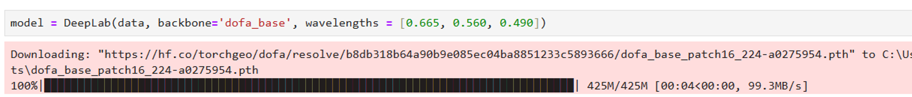
In this case, the exported data has an unsupported band. If you want to manually provide these values, the wavelengths parameter can be used. The following shows an example of manually providing wavelengths for an RGB image.
model = DeepLab(data, backbone = ‘dofa_base’, wavelengths = [0.665, 0.560, 0.490])
If you’re running this code for the first time, the weights for DOFA backbone will be downloaded and stored in a cache.
Fit the model
To train the model, use the fit() method, which uses the following arguments:
- epochs—Number of cycles of training on the data
- lr—Learning rate to be used for training the model
model.fit(epochs=10, lr=1e-4)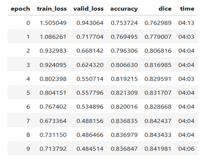
Visualize results and print average precision
The show_results() method can be used to visualize the results of the trained model.
model.show_results()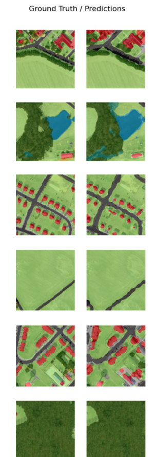
Save the model
Once the metrics and losses appear satisfactory, the trained model can be saved in the deep learning package (.dlpk) format, which is optimized for large-scale inferencing. This is the standard format used for deploying deep learning models on the ArcGIS platform. The save() method is used to accomplish this, and by default, the model will be stored in a subfolder within the training data directory.
model.save(‘deeplab_dofa_trained_model')
Conclusion
Geospatial foundation models like Prithvi and DOFA represent a significant development in the field of remote sensing. Their ability to learn generalizable representations from vast amounts of Earth observation data allows these backbone models to apply to a wide range of downstream tasks. By integrating these models into the ArcGIS ecosystem, users of all skill levels can now use these technologies.
Start exploring these new possibilities, experiment with the foundation models, and witness the enhanced performance they can bring to your remote sensing analysis.

Article Discussion: