Impervious Surface Mapping Using ArcGIS Pro – Part 2: Classification

Impervious surface maps are used for important storm water management operations such as helping to identify Best Management Practices for removing pollution from storm water runoff, determining storm water utility fees on a parcel basis, or flood control and emergency management planning.

The previous blog post about impervious surface classification discussed how to georeference your imagery in preparation for classification. Now that your imagery is properly registered to your landbase, this blog will focus on the science and art of multispectral image classification. In this case, you will perform impervious surface classification on the multispectral image. The result will be a thematic raster dataset classified into pervious and impervious surface areas.

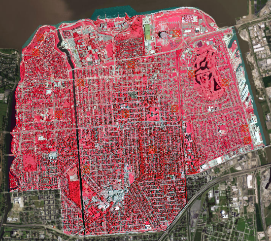
The first step is to display your image in a way that best discriminates your features of interest visually and analytically. For impervious surface features, you’ll want to display the imagery bands NIR (for vegetation), Red (for soil) and Blue (for urban features) as RGB.  You can use the Symbology pane and the Appearance tab to adjust your rendering.

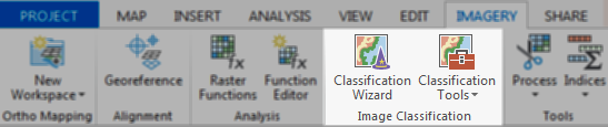
The Image Classification Wizard is a guided workflow that walks you through all the steps for image classification. To start the Image Classification Wizard, highlight the georeferenced layer in the Contents pane. Click on the Imagery tab to view two options in the Image Classification group: Classification Wizard and Classification Tools. Choose the Classification Wizard so you can perform the steps in an easy to follow guide.

The Image Classification Wizard is a pane with 8 possible steps (pages) to classify your image:

• Configure
• Segmentation
• Training Samples Manager
• Train
• Classify
• Merge ClassesAssign Classes
• Accuracy Assessment
• Reclassifier

Step 1: Configure

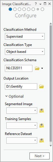
The first page in the Classification Wizard is the Configure step; its position in the workflow is indicated by the filled blue circle at the top of the wizard. The Configure page is where you set up the type of classification you want to perform and specify other files you will be using in your classification workflow. The parameters that are set on the Configure page  will affect which steps and pages you need to work with in the workflow.

You’ll want to perform a supervised object-oriented classification of impervious surfaces. The Classification Schema is a file that specifies the legend or classes that will be used. You can use an existing schema, or use the default schema and modify it – in this case use the default schema which is based on the USGS NLCD schema. You will create a new segmented image in the next step, so leave that parameter blank. The Training Samples input is a file that already contains polygon features of training samples. If you already have them, you can specify a file.  In this case you will create new training samples.

The last parameter is the Reference Dataset. This is the dataset of known classes that will be used to test the accuracy of our classification. Since this is a new classification we do not currently have a reference dataset and we will skip this step.  The topic of accuracy assessment will be addressed in part 3 of this blog series. Once you have filled out the parameters you want to specify, click Next.

Step 2: Image Segmentation

The Segmentation page will allow you to set up your image to be segmented into objects having similar color, shape and size characteristics. Use the three sliders to specify how you want to perform your segmentation. Generally, higher detail settings result in more discrimination between features and smaller objects, while lower settings result in more smoothing and larger objects. Because impervious surface features can consist of spatial objects having a wide range of size and shapes, the relative importance of the spectral information is greater than the spatial information. Usually the best practice for delineating impervious surface features is to set a higher value for spectral detail such as 16, and a lower spatial detail value such as 12.

The minimum size in pixels slider depends on your minimum mapping unit for your project.  So if you want to identify a small 8 foot x 8 foot shed and the resolution of your imagery is 50cm, then your minimum mapping unit is about 20 pixels. If you want to see what the segmented image would look like, click the Preview button.  You can continue to tweak your values until you are happy with the segmentation result. Leave the rest of the parameters as defaults and click Next. The segmented layer is created and loaded in the contents pane.

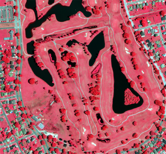
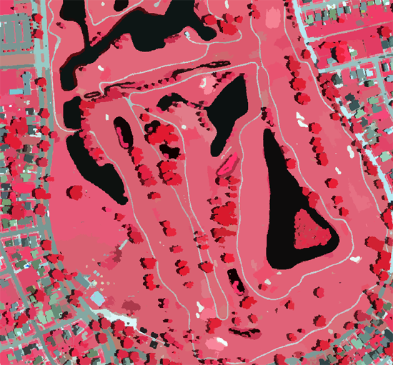
The top image is the multispectral source image dataset that you want to segment; the bottom image is the segmented image. The segmented image is more generalized by grouping similar neighboring pixels together into segments called objects.

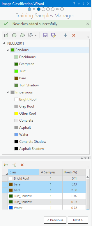
Step 3: Training Samples Manager

The Training Samples Manager is the third page of the wizard, and is populated with the default schema that you specified on the Configure page (NLCD2011).  First you will modify the default schema for Impervious and Pervious classes.

1. The default schema has 7 parent classes; delete all the classes except for Developed and Forest by right clicking on the class and selecting Remove.
2. Create an Impervious class by right clicking on the Developed class and selecting Edit Properties which opens the properties page.
3. Change the name to Impervious and select a grey color and click OK.
4. Edit the name of the Forest parent class to Pervious, and expand the Pervious parent class to expose the subclasses.
5. Delete Mixed Forest, and remove “Forest” from the Deciduous and Evergreen subclass names via the Edit dialog.

Next you will add additional subclasses to our schema.

1. Right click on the Pervious parent class and Add New Class named Turf, give it a green color and a value of 41 and click OK.
2. Add additional pervious subclasses named Bare and Turf Shadow, give them an appropriate color, and a value of 42 and 43 respectively.
3. Right click on the newly named Impervious parent class and select Add New Class and add the following impervious subclasses:  Bright Roof, Grey Roof, Other Roof, Concrete, Asphalt, Water, Concrete Shadow and Asphalt Shadow, and give them values of 21, 22, 23, 24, 25, 26, 27 and 28 respectively, and assign different grey intensity colors to each, except blue for water.

Note that water is often assigned to the impervious class for stormwater management purposes.  You now have your classification schema for impervious surface feature mapping.

1. To start collecting training samples, choose a subclass in the schema such as Bright Roof which activates the drawing tools.
2. Since we have a segmented image in the display, we can use the Segment Picker tool to choose entire segments.  Select the segment layer from the Segment Picker dropdown list to activate it.
3. You will need to zoom into the segmented image and choose an area that represents the class you have chosen. With the Segment Picker active, click on an area in the display to create a new training sample polygon segment.
4. Note – you may also turn off the segment layer in the Contents pane and collect training samples using the multispectral image in the display.
5. Click on the image and the corresponding segment will be captured as a training sample polygon.
6. Pan and zoom around to capture many samples for each class. Having a few training samples in each part of the image will provide good results in the classification phase. To help you navigate around and choose classes, use the keyboard shortcuts that are available. The C shortcut key is used to change your cursor into the Pan tool.
7. Make sure that you have a good number of samples and percentage of pixels or segments for each of the classes that you are classifying – 30 or more for each class is a good target. Depending on your image, you may have more training samples for a certain class since it occurs more often within the image.
8. To see the total samples and percentage of pixels, Collapse all of the training samples belonging to the same class.
9. Once you have a good set of training samples of each Impervious and Pervious subclass, click Next to move onto the next step.

Step 4: Train the Classifier

The Train page allows you to choose the type of classifier to use, and edit the parameters associated with that classifier. We will choose the non-parametric Random Trees classifier which has several advantages over other classifiers. It is one of the most accurate learning algorithms available in the discipline with reduced need for a normal distribution and similar sample size of the training sample data, gives an estimate of what variables are important in the classification, generates an internal unbiased estimate of error and runs efficiently on large databases.

Under the Segment Attributes dropdown, choose Mean digital number and Standard Deviation, and use the remaining default parameter values and then click Run. This step is a particularly computationally intensive part of the wizard and may take some time.  Two process are kicked off, the image segmentation and computing the training of the classifier, both are written to the output directory.

Once the training has been completed, the classification preview will be displayed. If the classification looks relatively accurate, you can click Next to save the classification.  If you feel that you want alter the training samples, you can click the Previous button and continue to edit training samples in the Training Samples Manager.  A rule of thumb is to collect training samples of misclassified features and assign the proper class to the training sample.  This approach refines the classification by focusing on correctly identifying misclassified features.  Once satisfied, click Next and then Run on the Training Samples Manager page to reclassify using the updated training sample file. Also keep in mind that you can always reclassify specific segmentspixels later on in the workflow.  Once satisfied with the classification results in the preview, click Next.

Step 5: Create the Initial Class Map

On the Classify page, you can specify the names of the classification output which will be saved to the Output Location that was specified on the Configure page. Once you have specified the output names, click Run to create all the classification outputs. This is another computationally intensive parts of the wizard, which may take a while to process.

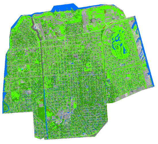
 Step 6: Merge Classes

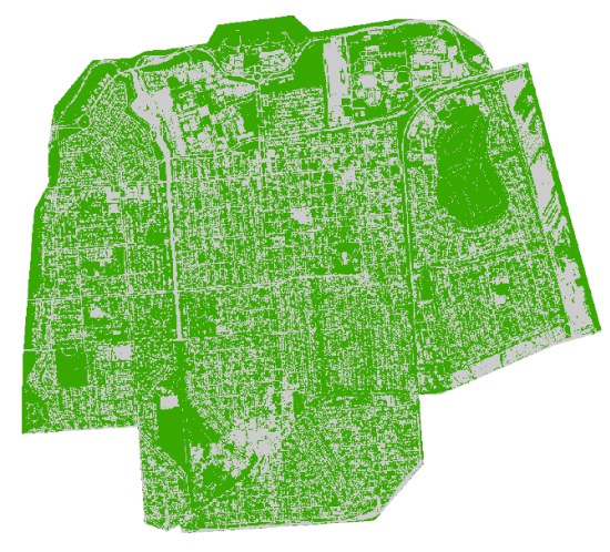
When the classification is complete, the thematic classified raster (see above) is created and is added to the Contents pane. Click the Next button to bring up the supervised Merge Classes page displaying a preview of the merged classes. Here you can choose to merge your subclasses into their parent class. Since we only want impervious and pervious surface features we can use the dropdown arrows to choose Impervious and Pervious as the new classes.  Click Next to generate the updated Impervious Surface class map and progress to the next page in the classification wizard.

Step 7: Reclassify

The Reclassifier page allows us to manually edit classes that are visually incorrect. You can use two types of tools reclassify incorrect pixels to the correct category. The purpose of this step is to fix a few misclassified pixels or objects, instead of re-running the entire classification wizard again. Use the Reclassify within a region tool to delineate a region where all the class polygons of one class type are reassigned to another class. Use the Reclassify an object tool to select a single class polygon and reassign it to another class.

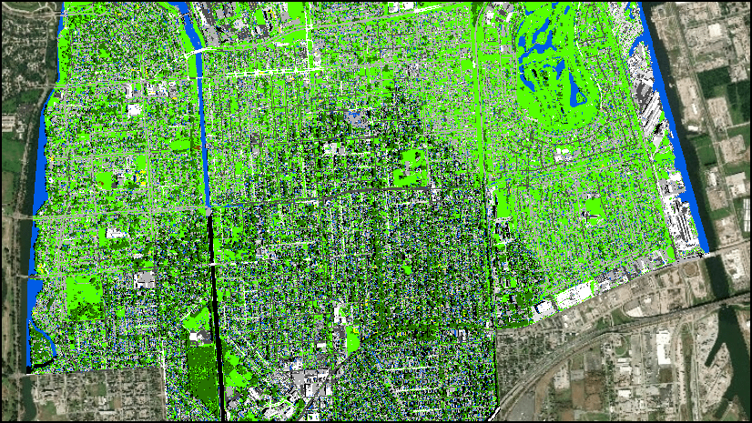
Once you have reclassified any incorrect pixels, click Run to generate and save the final classification output. Once you click Finish, you have completed all the specified steps in the Image Classification wizard. Now you can see the impervious surface classes as grey and pervious areas as green.

The Impervious / Pervious classification dataset is now ready to be used in your storm water management operations.

Accuracy assessment is a very important step in an analytical classification workflow.  The accuracy assessment step was skipped in this workflow in order to get a reasonable classification map quickly.  Accuracy assessment will be addressed in the final part of the Impervious Surface Mapping using Pro 1.4 blog series.

About the author

Jeff Liedtke

Jeff Liedtke is a PE and Documentation Lead for the Raster Team at Esri. He has a background in remote sensing, photogrammetry and image processing. Applying remote sensing techniques to provide valuable information for operational decision support applications is his passion.