Update: An extended technical article on this project is available here.
Authors: Dmitry Kudinov, Dan Hedges
Artificial Intelligence (AI), Machine Learning (ML), and Deep Learning (DL) have been quite popular in the recent years. Success stories from self-driving cars to medical imaging are filling the media. GIS is not falling behind: having efficient and intelligent tools will significantly cut costs of creating and maintaining GIS content and bring its quality to higher standards. Using AI in the transportation for planning and logistics, smart grid management, and more can increase productivity and improve safety.
What are these magic new tools?
Artificial Intelligence is a broad family of computer algorithms and methodologies which encompasses fields like Machine Learning (based on statistical methods), and, as we will be diving into here, Deep Learning (based on deep artificial neural networks). The unique and valuable feature of these approaches is the ability to learn and self-improve over time. If you are familiar with old-school image processing, you may remember hand crafting filter coefficients in order to identify features of interest from the data. Now, with deep convolutional neural networks (CNN), that is no longer needed; the network will learn these coefficients by itself during training, which is done by providing it with enough examples.
Introduction
Practitioners of urban GIS have long understood the need to think in the third dimension. The vertical nature of cities makes 3D GIS a necessity to answer many fundamental questions related to urban geographies, and to explain complex issues and deliver proposals to stakeholders and the public. The powerful suite of 3D tools and solutions available in the ArcGIS platform make this work possible, but a barrier to entry still exists in the ability of cities to create accurate base 3D content to do these analyses.
In this article, we will talk about an experiment we are conducting at Esri to explore ways to streamline the creation of 3D content using Artificial Intelligence. Specifically, we are using the power of the ArcGIS platform combined with a third-party deep learning framework, and high-end NVIDIA GPU cards to perform automatic feature extraction from remote sensing data.
In this collaboration with NVIDIA, using data from Miami-Dade County, we looked for ways to automate the manually-intensive process of creating complex 3D building models from aerial LiDAR data. Miami-Dade County graciously provided us with LiDAR point cloud coverage totaling over 200 square miles, and over 213,000 manually digitized roof segments of seven different roof types: Flat, Gable, Hip, Shed, Dome, Vault, and Mansard.
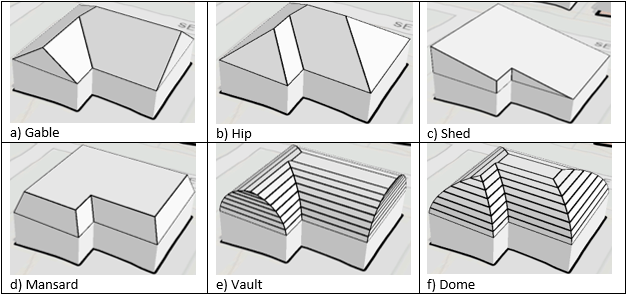
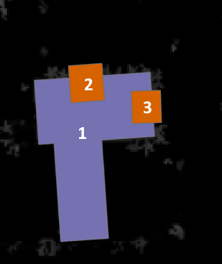
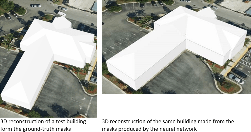
What makes this problem particularly fun yet challenging to solve is that modern architecture has generated roofs of a greater complexity than the above seven basic types. When these complex buildings are encountered, their roofs need to be split into multiple polygons so an accurate 3D model can be reconstructed. Here is a good example (Fig. 2):
The Experiment
Since the goal was to come up with accurate 3D representations of complex roof shapes, we first needed to answer a couple questions: what input format to choose for training data, and which neural network architecture to use – this is kind of a chicken and egg problem as one depends heavily on another. After some consideration, we decided to stay as close to the existing manual workflow as possible and convert LiDAR point cloud into a raster layer, which is how human editors performed this task.
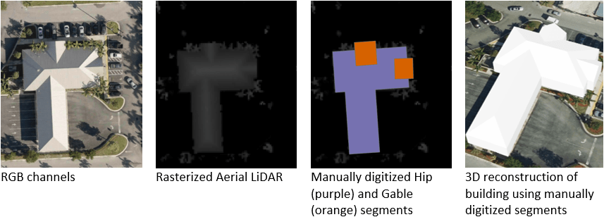
Human editors, in this case, did not use visible spectrum RGB channels to perform their job– only aerial LiDAR, as it is not always possible to have both sources of similar resolution properly aligned in space and time. Therefore, to match the existing workflow, our input format was a raster layer with 2.25 square foot resolution per pixel with a single channel representing pixel’s height from the ground level.
Once we decided on the input format, the second question was easier to answer. This task required not just detect a presence of a building, its bounding box, but also output a “mask” – a group of pixels uniquely identifying building’s roof segments (see Fig. 3).
In other words, we are dealing here with an “object instance segmentation” problem. Instance segmentation, for short, has recently enjoyed a lot of attention and contributions from academia and major companies, as it has a lot of practical applications in multiple areas from robotics and manufacturing, safety and security, to medical imaging. In 2017, Facebook AI Research published their first version of the Mask R-CNN, a state-of-the-art deep neural network architecture which outperformed all single-model COCO-2016 challenge winners on every task. We decided to evaluate the potential of the Mask R-CNN neural network in the remote sensing domain.
If we can train a Mask R-CNN to extract relatively accurate masks of roof segments and discriminate among the basic roof types, then with the power of existing ArcGIS Geoprocessing tools and Procedural rules, the workflow of 3D building reconstruction will be mostly automated, significantly reducing the amount of manual labor and bringing down the cost of 3D content creation.
Miami-Dade County provided us with a significant number of manually digitized roof segments as a polygon feature class. It took over 3,000 man-hours for human editors to manually digitize all these polygons. This is a useful baseline for the quantity comparison: how many roof segments can a single GPU extract per hour? Is it economical?
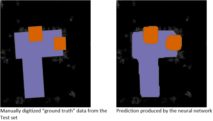
Quality assessment is another critical piece: how to define a metric which would give us a good indicator of predictions quality? For this we decided to go with traditional VOC-style mean average precision (mAP), i.e. evaluate how much produced predictions overlap with known ground-truth roof segments of the same class. There is a caveat in such approach though: the quality of the ground truth data (we used a subset of the manually digitized roof segments feature class which was not used in training) needs to be superb. In the case of our training data, a portion (roughly half) of the buildings in our dataset were designated to be digitized to a higher level-of-detail than other surrounding buildings, so there was the extra challenge of filtering out any images containing lower detail buildings from our test set. Nevertheless, we found that VOC-style mAP did a good job providing the baseline quality evaluation, which then was further verified with manual inspection of produced predictions.
For 3D reconstruction we used original LiDAR raster to post process produced predictions by further cleaning them and calculating floor count and square footage for each segment. Then we applied “Regularize Building Footprint” geoprocessing tool, and Procedural rules to restore building segments of corresponding height and roof type (Fig. 5).
After few months of experiments tuning hyperparameters and content of the training set, we came to the point where predictions were accurate enough (mAP of 0.49-0.51 on the Test set) so we could start manual inspections of the results, and work on applying 3D reconstruction steps.
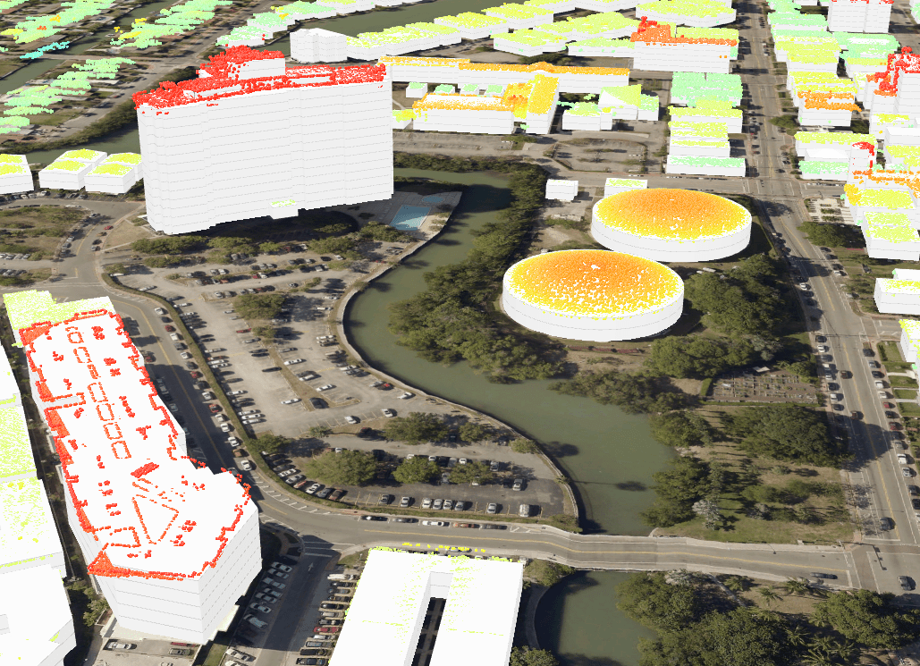
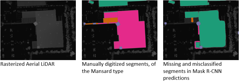
Of course, the predictions are not always correct, and often the neural network misses a roof segment, or sees only a piece of it, or incorrectly classifies the roof type (Fig. 7), but this certainly can be improved with further training. Moreover, from the numbers mentioned above, the human editor’s average rate is around 70 polygons per hour while digitizing these segments manually – in contrast, a pretrained Mask-RCNN neural network is producing up to 60,000 polygons per hour (!) from a single NVIDIA Quadro GP100 GPU, and this is certainly not the top limit – there is still a lot of room for throughput optimization.
Although we are still working on improving our implementation (Mask R-CNN detections are still far from being as accurate as the segments digitized by human editors), it is already safe to say that using AI for feature extraction from the aerial LiDAR datasets as a part of the workflow of 3D content generation is feasible and economically sound.
The Details
Training data
ArcGIS Pro 2.2 has a powerful set of tools which allows efficient creation of training datasets for artificial neural networks. Future versions will expand on this capability. In this experiment we used the 2.3 BETA version of the “Export Training Data for Deep Learning” geoprocessing tool which functionality was specifically enhanced to support creation of training datasets for instance segmentation (i.e. Mask R-CNN) problems.
The LiDAR raster we used for training has a resolution of 2.25 square feet per pixel, and after a few experiments we ended up using 512 x 512 tiles, about 18,200 tiles in the Training set total. Since the amount of training tiles was somewhat insufficient to do training as is, we used on-the-fly image and masks augmentation with affine transformations.
Still, straight-forward data augmentation did not help with another peculiarity which was in the diversity of the buildings in the given geography, as Miami-Dade County covers all sorts of zones: downtown high-rises, coastal resorts, rural single-family houses and duplexes, and manufacturing / warehousing sites. The variety of building heights was directly reflected in the input raster with its single 32-bit channel storing the heights in feet from the ground level. So, to amplify the useful signal before training, performed a local, per-tile normalization of the original 32-bit channel, converting its values into three 8-bit channels, effectively making a single-story building look equivalent to a 25-story resort. For each tile we compressed the original height to a 256-band value, and the other two channels were again 256-band normalized derivatives calculated along X and Y tile axis (SobelX and SobelY).
Training framework
We used TensorFlow 1.7 to run an implementation of Mask R-CNN neural network with a ResNet-101 backbone. Initially starting from the Imagenet pre-trained weights, we selectively trained fully-connected layers first in order to adapt them to our new classes, and then proceeded with the full network training for about 300 epochs (4 images per GPU) using two NVIDIA Quadro GV100’s connected with NVlink.
From the original Mask-RCNN (Kaiming He Georgia Gkioxari Piotr Dollar Ross Girshick. Mask R-CNN. 2017-2018) / FPN (T.-Y. Lin, P. Dollar, R. Girshick, K. He, B. Hariharan, and ´ S. Belongie. Feature pyramid networks for object detection. In CVPR, 2017) papers, our implementation was different only in sizes of anchors (10, 20, 40, 80, 160), and number of RoIs (1,000).
Inference architecture, tiling, virtualization
Once the Mask R-CNN model was trained to a satisfying state, it was time to integrate it with the rest of the ArcGIS platform, so it can be easily reachable from desktop and server products.
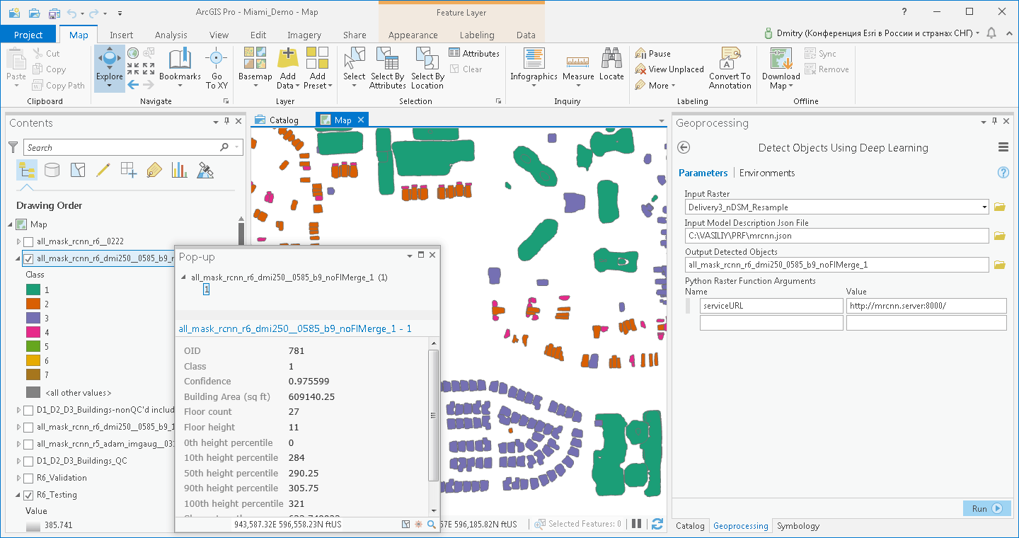
For the inference we used a client-server architecture which gives a clean separation of the roles of a GIS analyst and a Data Scientist, and allows for more efficient utilization of high-end GPU cards which, in such layout, can be used by multiple clients simultaneously. For this we leveraged the upcoming with ArcGIS Pro 2.3 new “Detect Objects Using Deep Learning” geoprocessing tool from the Spatial Analyst toolbox, which allows for invoking a custom Python Raster Function (PRF) – a python script, which is being run on the entire input raster according to a specific tiling schema defined by tile size and tile overlap.
When the PRF receives a tile, it compresses it to TIFF format and streams to a REST endpoint wrapping the Mask R-CNN model. Once the predictions are made, they are converted to a JSON feature set and returned by the REST endpoint. The response feature set gets passed by the PRF up, as is, to the ArcGIS platform where it is appended to the output feature class (or, in a future version of Raster Analytics, to a hosted Feature Service).
For the demo server to run the inference we decided to go with NVIDIA Tesla V100 (16GB) GPUs which are perfect not only for training and inference, but also for virtualization, when used with NVIDIA Quadro Virtual Data Center Workstation (Quadro vDWS) software, which efficiently splits GPU resources across multiple virtual machines. In our Esri UC-2018 demo platform we have two Tesla V100 cards with Quadro vDWS software powering four VMs: the inference service running on Ubuntu 16.04 LTS, and three Windows 10 machines with ArcGIS Pro 2.2 and 2.3 as inference clients running concurrently.
If you are at the 2018 Esri User Conference, stop by the ArcGIS Pro or Virtualization areas of the Esri Showcase to see a demo of the project!
Future Work
This is not a perfect solution See Fig. 5 as an example. It is not as sensitive as human editors (currently collecting by about 25% fewer roof segments in the same geographic area), but the good news is that there are multiple paths we can take to improve our results.
While the per-tile raster normalization to 3 single byte channels helps with reducing the amount of training data needed, there are downsides:
- Having a tall building in a tile tends to weaken the signal of fine structures as we are squeezing a large range into three 256-band channels.
- Limiting the size of the tile, as the “dynamic range” of the tile signal with such normalization drops inverse-proportionally to the square of the tile dimension.
We see two options to explore here:
- Use a logarithmic SobelX and SobelY.
- Significantly grow the training set and stay with the original 32-bit float, single band raster.
The former is fairly straight forward to implement and this will be done shortly, whereas the latter is may have more potential as will allow to grow the tile size more easily, which is important for efficient batch inference on the GPU side.
New Geographics Regions
We want to train and get the adequate prediction quality in other geographic regions. This experiment used data from Miami-Dade County, where ground elevation from the sea level is minimal and fluctuates very little. We trained our Mask R-CNN model with LiDAR raster with preliminary subtracted local elevation which introduces dependency on the accurate and high-resolution elevation model. We need to evaluate how much potential discrepancies between local elevation model and LiDAR data will affect predictions in more mountainous regions.
Including RGB Channels
Although it was mentioned before that it’s hard to find closely matching RGB and LiDAR data, it may not be such a big deal when we are dealing with a training set large enough. We will explore this direction as well. There are also known works (Benjamin Bischke, Patrick Helber, Damian Borth, Andreas Dengel. Overcoming Missing Modalities in Remote Sensing. NVIDIA GPU Technology Conference, 2018) where missing LiDAR channel was restored with an auxiliary Generative Adversarial Network using matching RGB input.
Raster Analytics Integration
We are actively working on enhancing the ArcGIS tools and integration frameworks which allow and promote effective and efficient ways of building and running an AI enabled GIS. One of the prominent pieces, currently in development, is the “Generate Table from Raster Function” geoprocessing tool that will enable running the above architecture in the ArcGIS Online or a private cloud.
Contributors: Thomas Maurer, Richard Kachelriess, Jim McKinney

Commenting is not enabled for this article.