By Aileen Buckley, Mapping Center Lead
I have been working on an online, multi-scale map of Yosemite National Park. This map will be incorporated into the World Topographic Map at map scales of approximately 1:9,000, 1:4,500, 1:2,000, and 1:1,000. From Yosemite National Park, we received elevation data at two grid cell resolutions: ten meter data for the entire park and 1 meter LiDAR data for seven or eight smaller areas within the park.
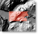
Figure 1 shows examples of these two data sets. The hillshade symbolized with the black to white color ramp was generated using the 10 meter DEM data, and the smaller extent symbolized with red tones was created using the LiDAR data.
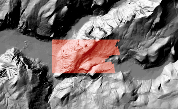
Figure 1: Examples of the two sets of elevation data that were used to produce hillshades for the Yosemite National Park area.
For this map, I am applying a transparency to my hillshade data rather than the vegetation because when I display the other layers under the hillshade, I can better enhance the depiction of elevation. (See figure 2.)
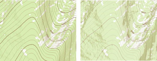
Figure 2: Comparison of the vegetation and contour data displayed on top of the hillshade (left), and the hillshaded layer displayed on top of the vegetation and contour data (right)
As you can imagine, if I have two sets of hillshade data that I am displaying transparently with other layers of information displayed underneath, the transparency becomes too opaque in areas where I have both hillshade data sets. The layers I am displaying under the hillshades become obscured and, from a map reader’s viewpoint, difficult to read. Also, as seen in figure 3, the color of the features change significantly when there are two hillshades being drawn on top of them. This causes the symbology across the map to vary when I really want it to be consistent.
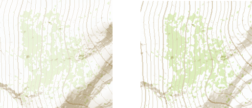
Figure 3: Comparison of vegetation and contour data displayed underneath the two hillshades (left), and vegetation and contour data displayed underneath only the LiDAR hillshade (right).
The solution to this problem is to clip the 10 meter hillshade where there is LiDAR data. The result is that the more detailed hillshade is displayed where the LiDAR data are available, and the coarser resolution DEM hillshade is displayed in all other areas.
The challenge with my data sets is two-fold: 1) The extents for the LIDAR data are irregular so I cannot just clip out regularly shaped rectangles, and 2) the raster data are at two different levels of resolution. Here’s how you, too, can overcome these challenges to clip out rasters of varying resolutions and irregular extents.
Step 1: Enable Spatial Analyst
First, enable the Spatial Analyst extension (from the top bar menu, click Tools, then Extensions, then turn on Spatial Analyst.
Step 2: Add the data to your ArcMap document
Next, add the two hillshade datasets to your ArcMap document.
Step 3: Set the raster analysis environment settings
Before you go any further, you should check some important settings that relate to raster processing. On the top bar menu, click Tools, then Options. On the Geoprocessing tab, click the Environments… button to access the geoprocessing environment settings (figure 4).
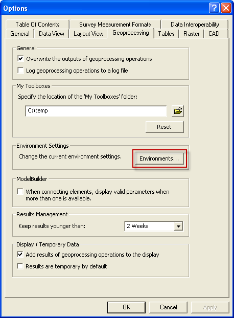
Figure 4: Accessing the geoprocessing environment settings.
Under General Settings, set the Extent to the coarser resolution 10 meter hillshade. Also set the Snap Raster to the 10 meter hillshade. Scroll down to find the options for Raster Analysis settings. Set the Cell Size to be the same as the coarser resolution DEM. Accept all these changes.
Step 4. Create a raster that represents the extent of the LiDAR data
In the Spatial Analyst toolbox, in the Math toolset, expand the Logical tools. The first tool you want to use is Is Null. What this tool does is to create a new output raster in which a value of 1 is assigned to cells whose value in the input raster is NoData and a value of 0 is assigned to cells that do have data.
The input raster for the IsNull tool is the LiDAR hillshade, and the output is whatever you want to call it – we called ours “IsNull_hd”.
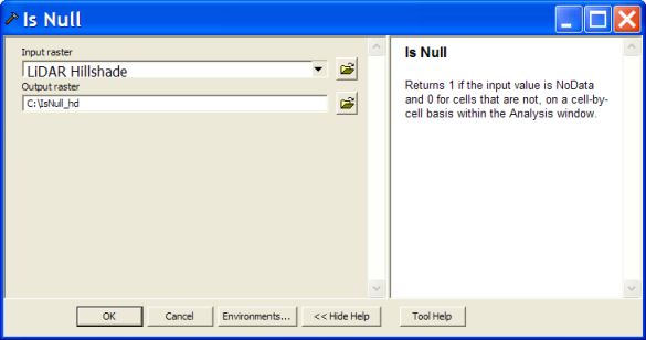
Figure 5: The input parameters for the isNull tool.
Recall that we set the analysis extent earlier in the Environment Settings. The result will be 0 where there is LiDAR data and 1 where there is 10 meter data, and the extent will be the same as the coarser resolution hillshade data (figure 6).
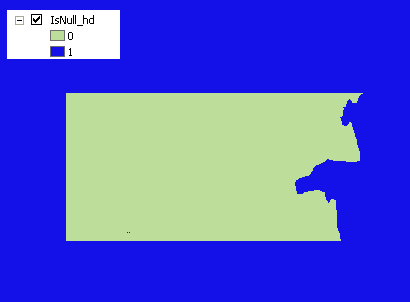
Figure 6: The output from the IsNull operation.
Step 5. Shrink the raster that represents the extent of the LiDAR data
Using the IsNull output, we now have to use the Shrink tool (this is in the Spatial Analyst Toolbox in the Generalization toolset).
Note: The reason that to use the Shrink tool is because we are working with dataset that have two different resolution and we want to avoid an edge matching problem in the final output. We tested several methods and found that the Shrink tool provides the best solution.
The Input Raster for the Shrink tool is the IsNull output created in the previous step. The number of cells to shrink by is 1 – the same resolution as the coarser resolution hillshade (remember that we set the analysis cells size in the Raster Analysis settings). The zone value is 0 – this is the area where there is LiDAR data (figure 7). The reason we are shrinking zone 0 is to make it a little smaller before the final step so we do not have gaps at the edges where the LiDAR data ends and the 10 meter data begins.
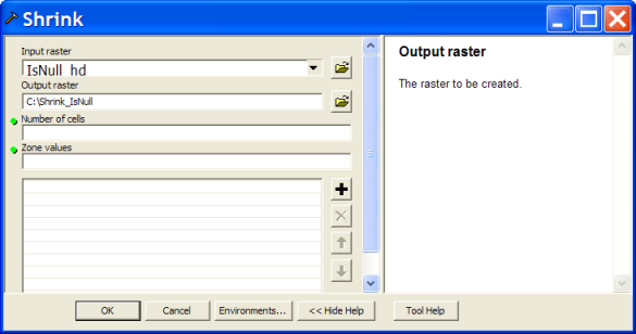
Figure 7: The input parameters for the Shrink tool.
The result will appear similar to the original IsNull output, but if you look closely, the extent of the LiDAR area (black) is slightly smaller than the original IsNull raster (pink), as seen in figure 8.
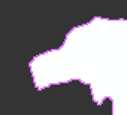
Figure 8: Cells with a value 0 in the IsNull raster are displayed in pink. The output from the Shrink tool is displayed in black. Predictably, there is a difference in size of one cell (at the resolution of the coarser raster) along the edges of the LiDAR extent.
Step 6. “Clip” the shrunken LiDAR extent from the coarser resolution DEM
The next step is to use the Con (conditional statement) tool (this is in the Spatial Analyst toolbox in the Conditional toolset) to create a new coarser resolution DEM that does NOT include the extent of the LiDAR data. In essence, what this tool will do is to create a new raster that has a value of NoData in areas where there is LiDAR data and has the original DEM values in areas where there is no LiDAR data. The conditional statement is, “If the cell in the shrunken LiDAR raster is not 0 (that is, it does not contain elevation data), then assign the cell in the output raster the same value as in the original DEM; otherwise, assign it a value of NoData”.
The input conditional raster is the output from the Shrink operation. The Expression is “Value > 0”, and the Input true raster or constant value is the 10 meter hillshade (figure 9).
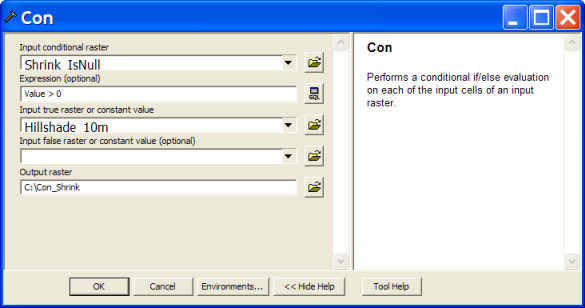
Figure 9 input parameters for the Con tool
The result is the 10 meter hillshade with a “hole” in it where the LiDAR data will be displayed instead (figure 10).
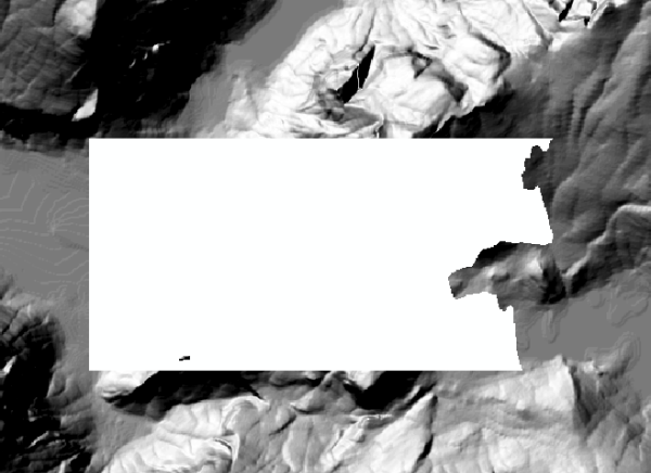
Figure 10: The output from the Con operation.
Step 7: Symbolize the output
The symbolized hillshades for the Yosemite National Park map are shown in figure 11.
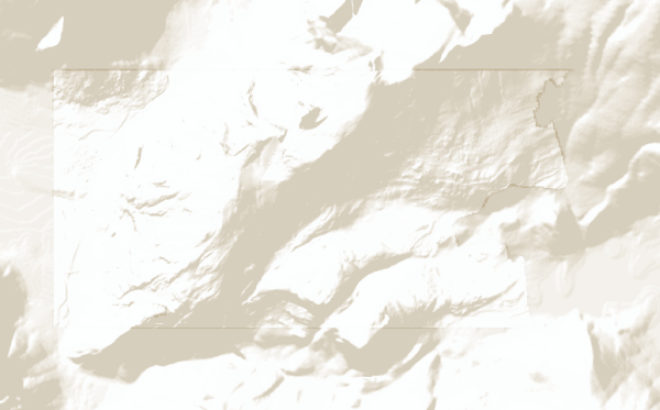
Figure 11: The final result in which the two hillshades are displayed with the same color ramp and the same level of transparency.
You can see a slight edge effect but this is a better alternative to a gap, which would happen if we did not shrink the output from the IsNull operation. Consider that we are displaying data UNDER the hillshade. If there were a gap, the colors of the underlying data would make the edge much more apparent. Our result mitigates that effect because although the one-pixel edge is darker, it has a transparency applied and the tonal variation will be softened by the color of the underlying data.
Since I am designing this map to be displayed at larger map scales, the overlap is preferred to white space. But, if you are using this approach for a map that will be displayed at a smaller map scale, the subtle difference may not be noticeable. If you decide the white space is not that apparent at the scale you are mapping, then you can skip Step 6 and go directly to Step 7.
Thanks to Nawajish Noman, Lead Product Engineer for Spatial Analyst and Geostatistical Analyst, and Aileen Buckley, Mapping Center Lead, for their help with this blog entry!

Hey y’all, great product so, is this dataset updated daily or is it static?
Thanks!
We have had a lot of fun putting it together. At this point we are planning on updating annually following the USGS’s national dataset release.
Can you please create a tutorial on how to first properly visualize the polygon
AreaFeatureswith respect to theElevation attribute(wish it had the depth attribute too) in a local 3D scene and then create an animation that shows the change in elevation and maybe even flow too.Regarding the use of the Elevation attribute in 3D, there is some instruction on that in the StoryMap linked below the video tour in the blog. Note that many smaller water bodies do not have an Elevation attribute. In these cases, copy the features you need from the service, then update any missing elevation values. To do this, you can just open a new Pro scene and hover the mouse over the copied lake or reservoir to get the Z information (at the bottom of the scene view window next to the mouse X/Y coordinates), then add a meter or… Read more »