Collection records from natural history museums provide a valuable source of biodiversity information that can be combined with environmental base layers from ArcGIS Living Atlas of the World, a curated collection of ready-to-use layers and other information products, to quickly examine the relationship between the distribution of organisms and the physical environment.
As an example of how you can use museum collection records and layers from Living Atlas to examine the distribution of organisms I queried an online portal, VertNet.org, for rattlesnakes in Riverside and San Bernardino Counties in Southern California. VertNet compiles collection records of vertebrate species from 394 museums and makes them available from a single easy-to-use webpage. With over 21,000,000 records VertNet provides a valuable resource for understanding patterns in nature. Many of the records contained in VertNet have location coordinates and are easily mapped with ArcGIS.
For this project I restricted the query to four species of rattlesnake. The four species have distinct ranges and appear to be limited to certain habitats. I removed records without coordinates and those with imprecise or questionable locations from the results yielding a list of 497 records for the western, red-diamond, western diamondback, and Mojave green rattlesnakes.
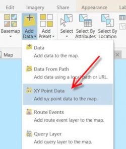
Map Your Points
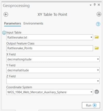
VertNet provides tab delimited text files that can be read directly into ArcGIS Pro. To map a data file downloaded from VertNet in ArcGIS Pro go to the Map Tab, select Add Data and then select X,Y Point Data on the drop-down menu. The XY Table to Point Tool opens. Set the file from VertNet as the Input Table and the X and Y fields should automatically populate with the decimallongitude and decimallatitude fields. Run the tool and the records are copied to a new feature class.
I knew I wanted to make a simple web application to share my work so I spent some time getting the new feature layer ready to publish. I deleted attribute fields that were not needed, added field aliases and improved the field names. I used the Field Calculator to do some light cleanup on the collector field and populate a common name field that I added and symbolized the layer.
Elevation and Slope
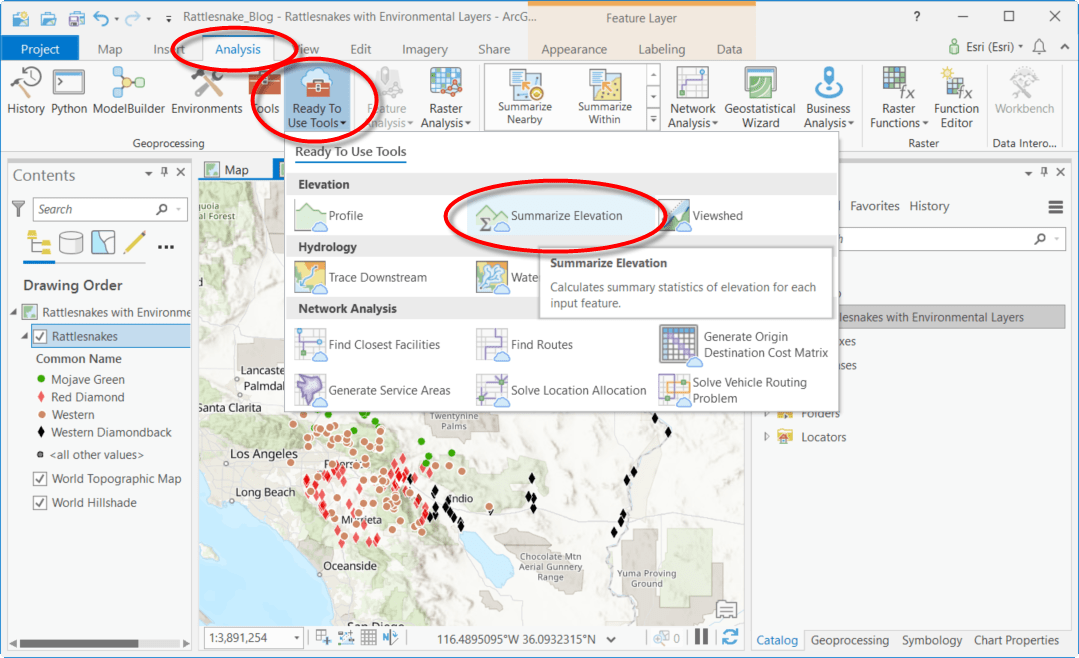
Southern California exhibits striking gradients in elevation from over 200 feet below sea level in the Salton Sink to the high mountain peaks of San Gorgonio (11,500′) and San Jacinto (10,800′). Since I suspect that elevation is potentially related to rattlesnake distribution I used the Summarize Elevation Tool in ArcGIS Pro to calculate elevation and slope for each point in my layer. The tool uses the Terrain imagery layer from Living Atlas to enrich your features. To use this tool click the Analysis tab > Ready to Use Tools > Summarize Elevation.
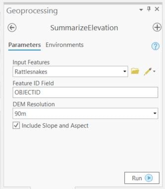
The Summarize Elevation tool creates a copy of the input features named “Output Summary” and adds 12 fields. I’m really only interested in two values so I used the Join Field tool to join mean elevation and mean slope to the original rattlesnake feature class. The Summarize Elevation tool adds a field named “ID” to join values to the “OBJECTID” field of the original table.
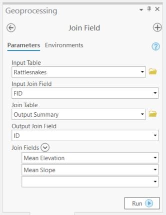
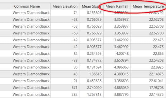
After running the Join Field tool I open the attribute table, scroll to the right and can see that the elevation and slope values are transferred to the original layer.
Add Rainfall and Temperature
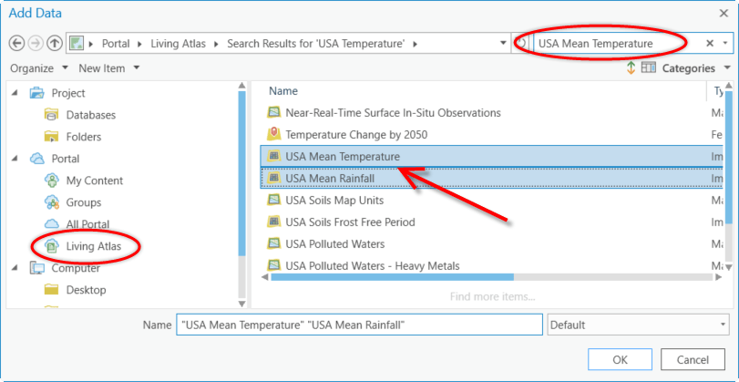
In this region areas closer to the coast and higher in elevation are much cooler and wetter than areas farther inland that are famous for their arid environments. To capture this variability I want to add values from two Living Atlas layers to my snake points. To do this I click Add Data under the map tab. In the Add Data dialog that opens I select Living Atlas under Portal on the left then type “USA Mean Temperature” in the search box at the top right. The two layers I want USA Mean Temperature and USA Mean Rainfall appear. I select them and click OK at add them to the map.
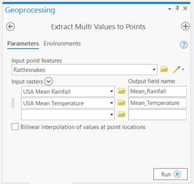
After adding the two layers to my map I used them as inputs in the Extract Multi Values to Points tool. Running this tool adds two more fields to our locations layer and populates them with mean annual precipitation and mean annual temperature for each point.
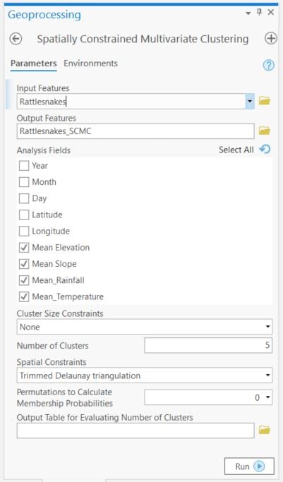
Spatially Constrained Multivariate Clustering
At this point we could make several maps using the environmental attributes we have added to to points. However, the ArcGIS platform provides access to sophisticated statistical tools that reveal patterns in the environment. One example is the Spatially Constrained Multivariate Clustering tool. This tool clusters data into geographically discrete groups that share similar environmental conditions. The settings that I used to group our points are below.
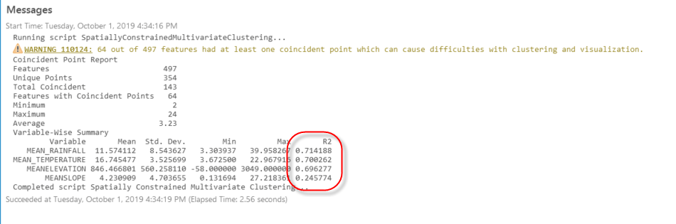
After running the tool, I clicked “View Details” at the bottom of the tool and expanded the details window to see the tool messages. The messages contain a useful variable-wise summary that includes a r2 value which provides an estimate of the variable’s ability to discriminate among our points. The values for temperature, rainfall, and elevation are all around 0.7 suggesting that they group the points well. Slope has a much lower r2 of 0.25 and does not have as much ability to group the points.
For more information on the tool’s output see How Spatially Constrained Multivariate Clustering works.
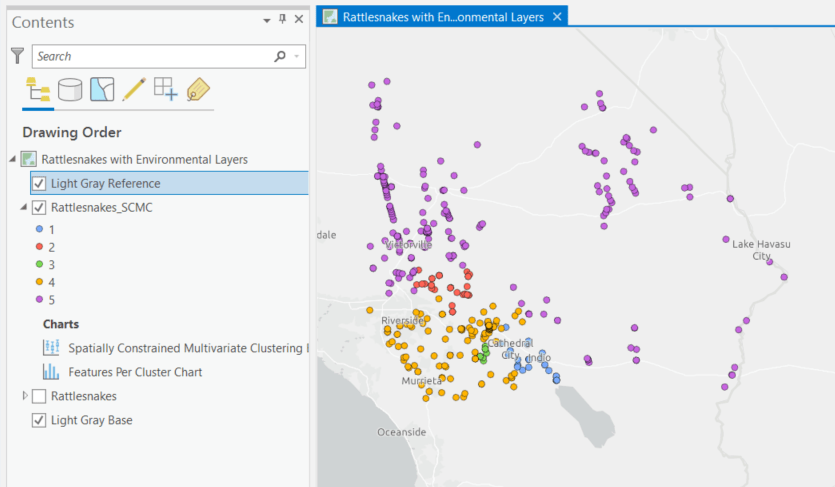
The tool clusters the points based on the attributes selected in the tool and adds a new layer and two charts to the map
The tool creates a chart labeled “Spatially Constrained Multivariate Clustering Box-Plots” in the map’s table of contents. This box-and-whiskers chart shows the relationship between each of the clusters and the four environmental variables. Note that colors on the chart match those in the layer’s symbology.
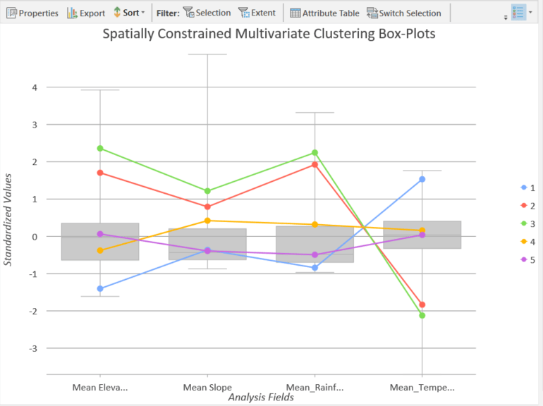
The chart reveals several patterns, for example groups 2 and 3, the red and green lines, are found at higher elevations, areas with higher rainfall, and areas with lower temperatures compared to the other three groups. These two groups correspond closely to populations of the western rattlesnake, a species often associated with cooler more northerly habitats. In this part of Southern California they find suitable habitat in the cool, relatively moist, mountainous, high-elevation areas. Note that the slope for these groups is also higher than the other three reflecting the species’ rugged mountain habitat.
Similarly from the chart you can see that group 1 is lower, drier, flatter, and hotter than the other four groups. This cluster stretches from Palm Springs southeast across the Coachella Valley to the Salton Sea. Twelve of our records have elevations below zero and all cluster in this group. This extremely hot, arid region is home to the western diamondback rattlesnake and records for this species dominate group 1.
To provide a way to share and explore my results I joined the Cluster ID value to the rattlesnake locations using the Source_ID field and published a hosted feature layer from ArcGIS Pro.
The application below contains the same rattlesnake layer used in the application at the beginning of this blog but symbolized with group rather than species name. The rainfall layer is in the background. You can use the application to explore the environmental layers used for the analysis. Turn layers off and on by clicking the layers button near the top left of the application. A layer with the snake species symbology is also included for comparison to the groups.
This analysis shows what you can do with Living Atlas resources that are available and ready for you to use. With powerful built-in tools like Forest-based Classification and Regression and EBK Regression Prediction plus access to extensive libraries for species distribution modeling in Python and R you can create sophisticated models and share your results in intuitive web-based applications.
Red-Diamond Rattlesnake photographs from the California Department of Fish and Game

Commenting is not enabled for this article.