ArcUser Online

Planning Forest Operations
A rule-based spatial DSS built with ModelBuilder
By Daniele Lubello, University of Padova, Italy

This article as a PDF .

Improving operational efficiency through better management is one way that the Italian forest industry can enhance its competitive position. The GIS-based model, described in this article, supplies decision support system (DSS) for forest managers.

The FOpP Defining Skidding Systems dialog box. Each parameter for the tool is described on the right side.

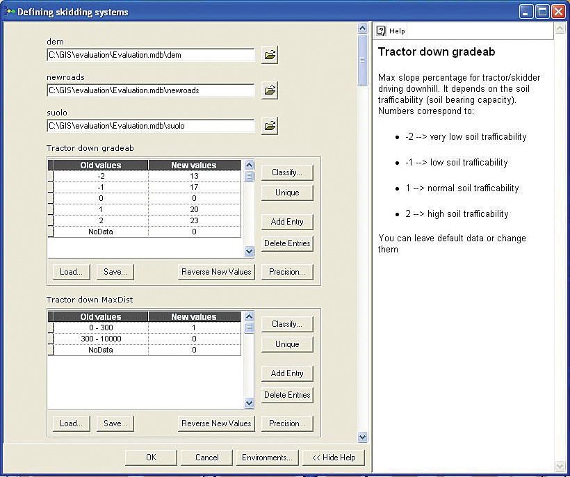
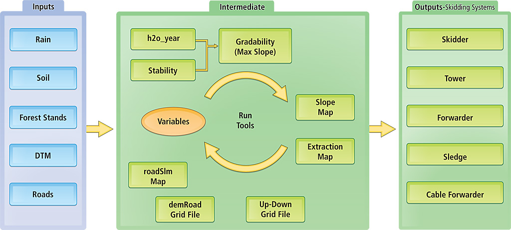
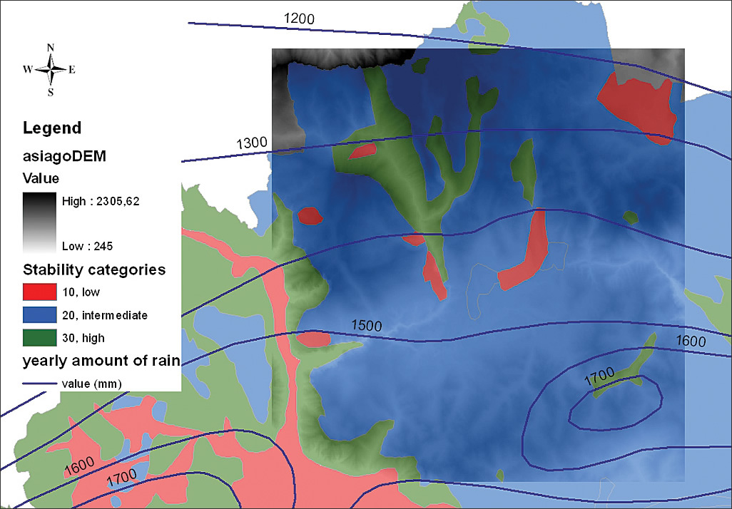
Initially, DSS applications and modeling were primarily developed to meet military needs and estimate the load bearing capacity of soils for off-road vehicles. The approaches were later applied to agriculture and forestry. Accessibility maps and analysis for planning forest operations have prevented damage to wetland soils and ecosystems.

DSS models for steep Alpine areas, where forest management is concerned with wood production, hydraulic and soil protection, biodiversity conservation, and tourism, require complex analysis. For example, the density and size of remaining standing trees have a high influence on skidding operations. In addition, planning models must consider not only environmental and stand factors but also the prevention of soil compaction damage. Recent research has considered the problem of optimizing different skidding systems but did not incorporate user-friendly GIS models that could be easily shared between researchers.

The Forest Operation Planning (FOpP) model defines a forest area that allows a specific skidding system can be used based on its technical capabilities and determines where that system should work to reduce operational costs and increase the value of wood.

ModelBuilder was chosen to build the FopP model because it is a powerful tool for building models that does not require knowledge of any programming language. The model can be created in a step-by-step fashion. The model dialog box allows results to be checked or errors verified immediately and environment settings used to ensure all data is in the same projection. For complicated models, outputs can be stored in a geodatabase and intermediate files can be deleted at the end of the process.

To simplify procedures and reduce the running time, the FOpP model was split in two parts: Defining Skidding Systems and Systems Optimization and Costs. Defining Skidding Systems creates one feasibility map for each skidding system. Systems Optimization and Costs establishes technical and economic preferences for the skidding system. Opening the model by double-clicking on its icon, ArcToolbox allows the user to set parameters and run the tools.

Defining Skidding Systems

The first step determines gradability classes using soil and rain shapefiles as inputs. The soil polygon shapefile is converted into a grid file based on soil classification (e.g., minerals and pH) and reclassified into three soil stability classes: high, normal, and low. The output file is named stability. The rain polyline shapefile is also converted to a grid file and reclassified into four classes according to the average amount of rain per month and year with assigned values between 10 and 40. Classes are defined based on average precipitation for an Alpine climate. The output file is named h2o_year.

Functional layout of the process for defining skidding systems

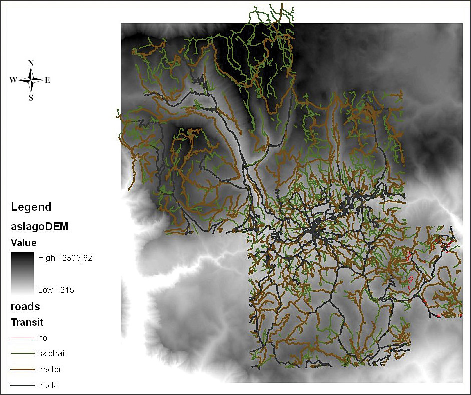
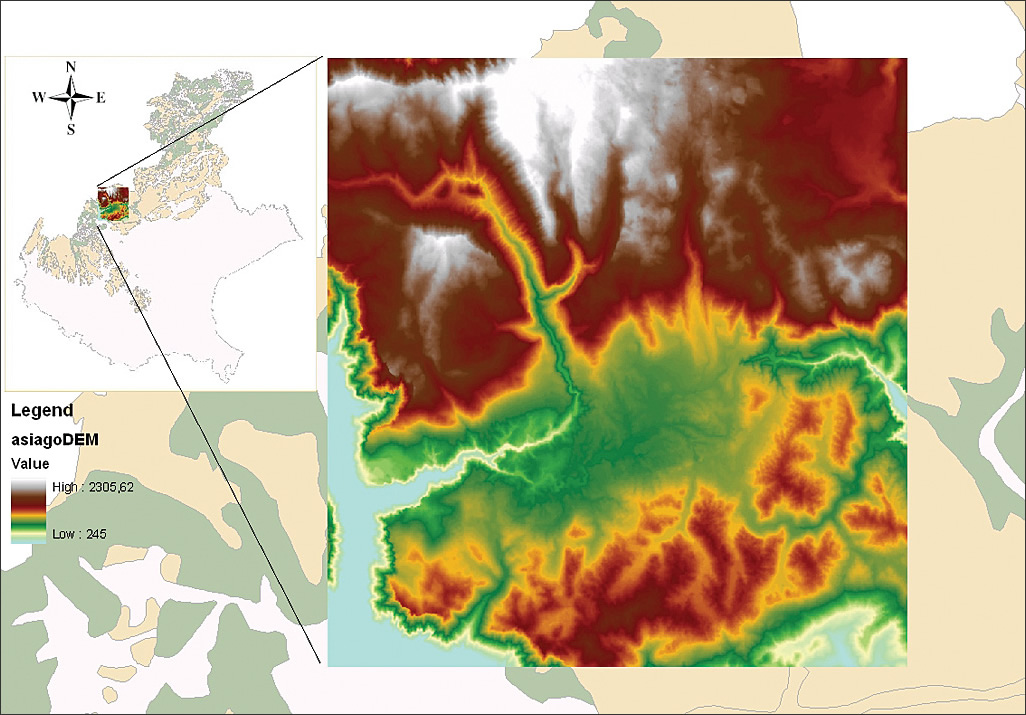
The stability and h2o_year grid files are summed using algebraic tools and reclassified into four gradability classes: high, normal, low, and very low. Using these classes, the maximum slope that will allow off-road systems to travel without slipping can be determined. Maximum slope values are set as model parameters so they can be adapted by the user via the model interface.

Slope, extraction distance, and uphill or downhill skidding direction maps are then created. The slope map is created from the digital terrain model (DTM) using the Slope tool in the ArcGIS Spatial Analyst extension tools in ArcToolbox. Values are calculated as percentages.

The extraction distance is generated from the roads shapefile using the Euclidean Distance tool in Spatial Analyst. Although the maximum distance may be changed by the user, the default value is 1,500 meters.

The evaluation of uphill and downhill skidding direction is more complicated. Vector roads are converted to a grid file. Only truck and tractor roads are used for this analysis; skid trails are not considered. The roads grid is used as a mask to extract values from the DTM (i.e., the RoadSlm map). Using the Path Distance allocation tool, values for each road cell are spread over the area at an equal distance from other roads (i.e., the demRoad grid file). Using the map calculator, DTM values are subtracted from demRoad values to create a map with positive and negative values. The Up-Down grid file is calculated by reclassifying the values. Positive values correspond to the uphill road side (downhill skidding direction) and negative values correspond to the downhill side.

The model makes a cell-by-cell evaluation for both skidding directions according to the technical limits of each machine in terms of maximum slope and distance, which are incorporated as model variables. These variables can be modified by the user for specific machines or situations.

	Inputs to the Define Skidding Systems tool include forest, soil and rain, road network, and elevation data layers.

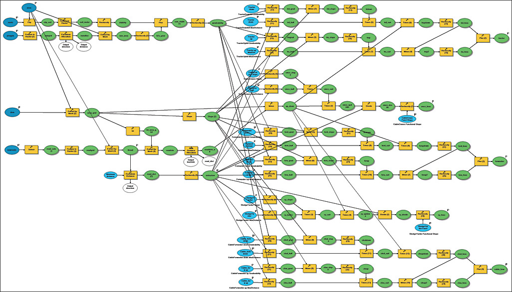
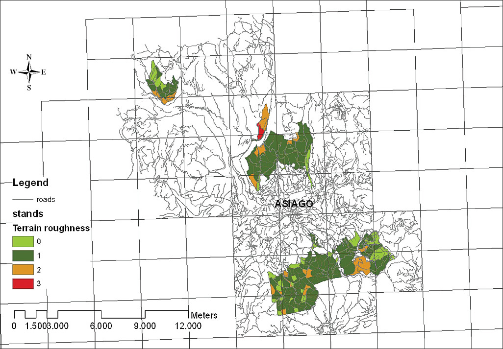
Setting these technical limits lets the model determine feasible areas for each selected skidding system. The evaluation of feasibility maps is quite similar for off-road and cable systems. Output maps distinguish the skidding direction. For cable systems, the model verifies that the average inclination from each cell to the nearest road is sufficient for the system to operate.

Systems Optimization and Costs

The second part of the model overlays five maps for skidders, forwarders, tower cranes, sledge yarders, and cable forwarders for two types of analysis: technical and economic. The algorithms for both analyses start from a basic classification of the timber stand based on terrain roughness and yield. The terrain roughness is a limiting factor for the movement of machines off road. Yield influences the productivity (and attractiveness) of certain systems.

For example, if the yield for an area is estimated at less than 48 cubic meters per hectare, relocating a big machine such as a forwarder isn't justified, and a tractor with winch would be used instead. Systems are ranked—tractors and mobile cable cranes are at the same level, the forwarders and sledge yarders are at another level, and cable forwarders occupy another level. The basic classification determines the choice of system.

Starting from an input stand shapefile, terrain roughness is reclassified into four levels (10, 20, 30, 40). The yield is reclassified into three levels (0, 1, 2). The two maps are summed to create stand classes. The most appropriate system is assigned to each stand class, and other systems that could work are also indicated. When the model makes the map overlay, it selects systems in that order.

The technical evaluation algorithm starts with the five systems maps and performs an overlay, taking into account the stand classes defined in the previous process. While the procedure looks complicated, only two Spatial Analyst tools are used—the Reclassify tool and the Single Output Map Algebra tool. The number of systems and the distinction between uphill and downhill extraction make the calculation time lengthy. Calculating the entire model takes approximately 40 minutes, depending on the size of the area and the grid cell chosen. The output map for this analysis also highlights areas that cannot be reached either because they are too far from roads or are too steep.

The wood supply basin between Italy and Slovenia generated by considering the maximum difference in supply cost between the two terminals of � 2�/m3

Through the model dialog box, the user can set average costs and the efficiency of the selected skidding systems. The model uses this information to make a simple cost evaluation. The technical map is reclassified, and costs are calculated on a cell-by-cell basis to provide both per cell and per cubic meter values. Outputs are grid maps and database tables containing statistics for the forest stand. Minimum, maximum, average, and total costs are calculated and are strictly dependent on the yield distribution and the choice of systems.

Because each skidding system has a different level of productivity and cost, the associated values for each cell are unique. The optimization algorithm starts from this assumption and selects the cheapest system using the Spatial Analyst Cell Statistic tool, which chooses the minimum value between different overlaying grid files. This produces a cost_select map that is compared with systems cost maps to assign to each cell the corresponding system. Each of the maps (one for each skidding system) is summed and reclassified to produce an optimal systems map. This map is similar to the technical systems map but may eliminate less efficient systems. For example, a tractor system might not be included because its low productivity makes it one of the most expensive systems.

Inside the optimization method, the cost calculation uses specific systems functions, which are estimated from references and field surveys and correlate productivities with skidding distance from forest roads. Values decrease exponentially with increased skidding distance. After this calculation, the duration and cost of skidding operations are known. These values are transformed in cost in euros per cubic meter, and optimized output cost maps are created.

An interesting model process estimates how much wood will be skidded to each forest road section and calculates the average cost of this process. The results of this analysis may be interpreted to determine the effect of building a new road or estimate the cost of transporting wood (primarily using trucks) in terms of the road maintenance that will be required.

Implications for Forestry-Wood Chain Analysis

The results of this model are a good starting point for the analysis of the forestry-wood chain. By adding felling and other administrative costs, it is possible to estimate total operational costs and compare them with wood market prices. A forest manager can determine if operations will be profitable or evaluate the effect of sylvicultural management, as related to yield, on total costs.

Through a network analysis, transportation costs can be estimated providing good logistic information about the catchment area related to the location of terminals or industrial areas. For more information, contact Daniele Lubello at daniele.lubello@unipd.it.

About the Author

Daniele Lubello is a private forestry consultant working on forest and road planning. He has spent the last three years as a doctoral student at the University of Padova, Italy, in the Forest Operations Management Unit (TeSAF department). He developed this model as part of a project for defining an integrated way of planning sustainable forest cuttings and machinery operations.

Learn More

Esri offers a free Web training seminar, Geoprocessing Using ModelBuilder, a Web course, Learning ArcGIS Spatial Analyst, and an instructor-led course, Working with ArcGIS Spatial Analyst.