ArcUser Online

Under Construction
Building and calculating turn radii
By Mike Price, Entrada/San Juan, Inc.

This article as a PDF .

Fog Lines and Tangents

Past exercises in this series used speed limits, global turns, and slope to modify transportation network travel times. This exercise addresses the need for modeling tight turns on narrow winding roads when mapping rural, mountainous terrain.

Although I challenged my students at Bellingham Technical College to develop a fast, repeatable way to calculate radii for turns on existing mountain roads, we hadn't made any progress until one day last spring. I was driving home from a meeting where radius turns were discussed when my eyes began following the fog line on the right side of my highway travel lane. In Washington state, the fog line helps a driver track the roadway edge during limited visibility. I was fascinated by the way the line would appear straight, then curve, then straighten again. Sometimes, the line would even transition from a curve to the left, to a curve to the right, and back to a left curve again, without straightening.

I thought I might be onto something. I realized that if I could map these inflection (or tangent) points through each curve, ArcMap would calculate the length of its connecting chord. I also thought that I could use ArcMap to model and measure the distance from the turn chord to the farthest point away from the line and even calculate the travel distance around the curve.

After trying all types of geometric constructions using circles, ellipses, and irregular curves, I discovered a simple formula that required only the chord length and the perpendicular distance from the chord to the maximum curve extent (a line called the Middle Ordinate). I tried this formula on several curves, and it worked. On the Internet, I found the same formula on several engineering sites. I realized that it would be possible to draw and measure these lines in ArcMap and use this simple formula to determine the radii of a number of curves.

An Overview of the Exercise

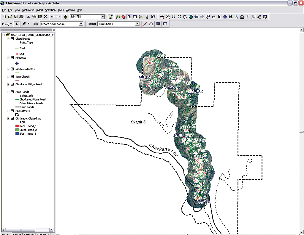
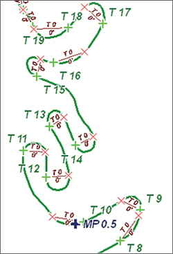
This exercise was simplified by preselecting tangent points for the 47 significant curves on Chuckanut Ridge Road.

This exercise introduces a heads-up methodology for constructing and measuring line segments and calculating turn radii on a carefully digitized road centerline. In the next portion of the workflow, the road is broken into curves and straight lines. Once each curve contains its own radius, travel restrictions and impedance parameters may be developed and used for response modeling.

This methodology consists of five tasks.

Task 1: Identify and assign the start and endpoints of each curve—the point at which the road polyline transitions from straight to curved or tangent.

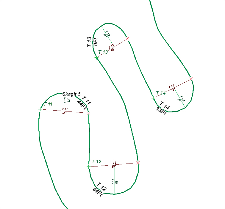
Task 2: Construct a two-node polyline (the Chord) to connect the curve points. Calculate its length in project units and assign each chord a unique, sequential number.

Task 3: Construct the Middle Ordinate, a two-node line perpendicular to the Chord, and intersecting the curve at its farthest point from the Chord. Assign a unique number for each curve in the Middle Ordinate table and calculate its length.

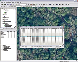
To zoom to the beginning of Chuckanut Ridge Road, select the CR MP 0.0 1:500 bookmark.

Task 4: Break the road polyline into curves and noncurves. Calculate the lengths of all road segments and assign each curve a turn number matching its Chord and Middle Ordinate.

Task 5: Join the Chord and Middle Ordinate tables to road segments. Populate the Chord and Middle Ordinate length fields for each curve. Finally, apply the curve radius formula to calculate the radius of all curves and make a map.

The Study Area: Chuckanut Ridge

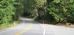
Chuckanut Ridge is a private, gated community on Chuckanut Mountain in Bow, Washington, an unincorporated community in northwestern Skagit County. It is the second Firewise USA Community [Firewise Communities/USA, recognized by the National Fire Protection Association, are small, cohesive neighborhoods and towns within the Wildland/Urban Interface acknowledged for homeowner involvement and commitment to minimize home loss to wildfire.] organized in Washington state. Chuckanut Ridge Road, a single hard-surfaced 16-foot-wide road, accesses a handful of private homes scattered up the mountain. It starts at Chuckanut Drive and climbs from an elevation of 160 feet to nearly 1,600 feet in just 3.5 miles. Its average slope is nearly 11 percent, and its many twists and turns include at least 20 switchbacks or sharp S-turns. In addition, some curves actually tighten within a turn, creating an additional driving hazard.

Skagit County Fire District 5 provides fire and emergency medical service to Chuckanut Ridge. The district built a new satellite station and is outfitting a specially designed fire engine for response up the steep hillside and along Chuckanut Drive.

Getting Started

The chords will be numbered to match the Chord Points so build them sequentially. When finished, turn off the background image and inspect the chords.

To start this project, download the sample dataset (Chuckanut.zip). Store this file near the root directory of the drive and extract the data and allow the creation of subfolders. Open ArcCatalog and navigate to the new Chuckanut folder. Inspect the shapefiles that will be used for this exercise.

This data is registered in Washington State Plane North American Datum of 1983 (NAD83) High Accuracy Reference Network (HARN) North Zone. Units of measure are U.S. Survey Feet. Notice that there are also several layer files that will be used to reference and symbolize data.

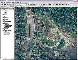
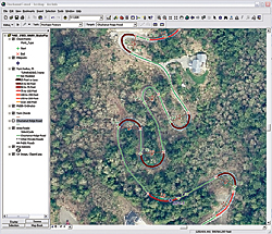
Preview the attribute tables for Chords1.shp and MidOrd1.shp in ArcCatalog and verify that both tables contain no values and are ready to hold the results of calculations. Navigate to \Chuckanut\JPGFiles\WASP83NFH and inspect the background image. This graphic was registered, resampled, and clipped from a high-resolution image provided by Skagit County GIS. Although it is pixilated, this image can make the relationships between residents, vegetation, and the access road more apparent.

Task 1: Understanding Curves

Describing the curves on Chuckanut Ridge Road will require locating the points on both ends of each curve where the road centerline transitions from straight to curved. In a node-based polyline, this location is best represented by a single vertex where succeeding line sections are no longer lined up. If this curve were ideal, a straight line would touch it at only one point; the line would be tangent to the curve. In practice, although few curves are ideal, it is still possible to visually select two vertex points for each curve where the tangent begins and ends.

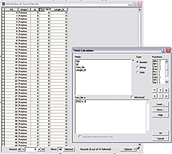Use the Field Calculator to populate the Turn_No field by numbering the chords using the simple formula [FID] + 1.

This exercise was simplified by preselecting tangent points for the 47 significant curves on the road. These points include start and end attributes and are numbered from 1 to 47.

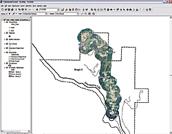
1. Start ArcMap and open \Chuckanut\Chuckanut1.mxd. Fire District 5, area roads, Chuckanut Ridge Road, and its mileposts are all displayed over an aerial image of the study area. Zoom in and look around.
2. Navigate to \Chuckanut_Safe\SHPFiles\WASP83NFH and load the Chord Points, Turn Chords, and Middle Ordinates layer files. Open the table for each layer and notice that the Chord Points table is fully populated while the other two tables are empty.
3. To make navigating around the map easier while working the exercise, several bookmarks were added to the map document. From the Standard menu, choose Bookmarks > Manage and select CR MP 0.0 1:500, located at the bottom of the list. The map zooms to the beginning of Chuckanut Ridge Road.

Notice that the road contains many vertices, typically spaced less than 20 feet apart. Modeling these curves requires carefully densifying the polyline. Carefully inspect the road centerline and observe how the Chord Points are placed. These Chord Points will be connected in the next section to build Turn Chords. Save the project.

Task 2: Constructing Chords

Number curve segments to match the Turn numbers by selecting a turn segment and entering its number in the Chuckanut Ridge Road attribute table in the TURN_NO field.

1. Choose View > Toolbars > Editor to load the Editor Toolbar and start an edit session. In the Editor toolbar, set the task to Create New Feature and make Turn Chords the target. On the Editor toolbar, in the Editor drop-down menu, choose Snapping and set the snapping layer to Chord Point vertices. In the Editor drop-down menu, choose Options and set the Snapping tolerance to 50 map units.
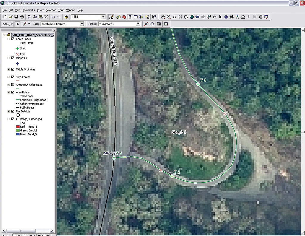
2. To build the first chord, activate the Sketch tool and use the cursor to snap to Chord Point T1, the green crosshair located at MP 0.0. Extend the line to the next red "x" and double-click to terminate the chord. Notice that it will be immediately labeled with zero values. Continue moving up the road, building Chord 2.
3. Hold down the C key to access the Panning tool and move along the road. To speed up this process, use the mouse wheel to zoom in and out. Build each chord in order from T1 to T47. The chords will be numbered to match the Chord Points so build them sequentially. When finished building the chords, turn off the background image and inspect them.
4. The next step is to add a Turn Number and the chord length. Open the Turn Chords table and verify that the FID field contains a continuous series of values that starts with 0 and ends with 47. If the FID values are not in a continuous sequence, renumber the chords to match the Turn Point series.
5. Right-click on the Turn_No field and choose Field Calculator. Use the Field Calculator to number the chords by using the simple formula [FID] + 1 to populate the Turn_No field. Make sure the box next to Calculate Only Selected Fields is unchecked. These chord lengths will be joined to the road set, so make sure the numbers begin with 1 and end with 47.
6. Now, let's calculate each chord's length in U.S. Survey Feet. Right-click on the Length_Ft header and choose Calculate Geometry. In the Calculate Geometry dialog box, set Property to Length, use the coordinate system of the data source, and choose Units to U.S. Feet. Notice that this operation yields length values rounded to two places. These values appear on the map just below each turn number.
7. Make sure all the numbers are in order and that lengths are reasonable and save the map. Don't end the edit session because the next step is building the Middle Ordinates.

Task 3: Modeling the Middle Ordinate

Select Ridge Road, change to the Split Tool, click on the end point of the Turn Chord, and left-click once to split the line. Reselect the next uphill portion of the road, grab the Split Tool, and repeat the process.

In a perfect curve, the Middle Ordinate is a two-node polyline extending perpendicular from the Turn Chord to the farthest point out on the curve. Use the CR MP 0.0 1:500 bookmark to return to the extent at the beginning of Chuckanut Ridge Road.

1. On the Editor toolbar, change the Target from Turn Chords to Middle Ordinates. Keep Create New Feature as the task.
2. Under Snapping in the Editor toolbar, check the boxes for Turn Chord edge and Chuckanut Ridge Road vertex. Since the Middle Ordinate is often very short, change the Snapping tolerance to five map units.
3. Starting with Turn 1, use the Sketch tool to draw a polyline connecting the farthest point on the curve to the Turn Chord. Slide the second point along the chord until it appears perpendicular. Double-click to save the feature. Continue up the road, building a Middle Ordinate for each curve.
4. Once all the Middle Ordinates have been sequentially built, save the project.
5. Number the Middle Ordinates to match each associated turn using the Field Calculator. Calculate the Middle Ordinate lengths using Calculate Geometry (the same procedure used for the Turn Chord table). Use CR MP 0.5 1:1,500 to zoom in, turn the image back on, and inspect the map. Be sure that all vectors are properly numbered. Save the edits and the map. This might be a good point to stop and take a break.

Task 4: Splitting Lines and Separating Curves

Join the Chuckanut Ridge Road attribute table with the Turn Chords table using the Turn_No field.

Now it's time to split the Chuckanut Ridge Road into curves and straight segments using the Turn Chord endpoints to locate each split point. When performed manually, this task is quite rigorous. If we could intersect all chords with the road, this would be an easy task. However, using the Chord Points and a special VBScript, the road can be split into curves and straight-line segments. See the accompanying article, "Road Repairs: Splitting Polylines with Visual Basic Scripting," for detailed information on how this procedure is accomplished.

1. Navigate back to Bookmark CR MP 0.0 1:500 once more. Make Chuckanut Ridge Road the Target layer and the only selectable layer and change the Task to Modify Feature. Change the snapping layer back to Chord Points vertex (or alternately, Turn Chords end). Start editing again and reset the Snapping tolerance to 50 map units.
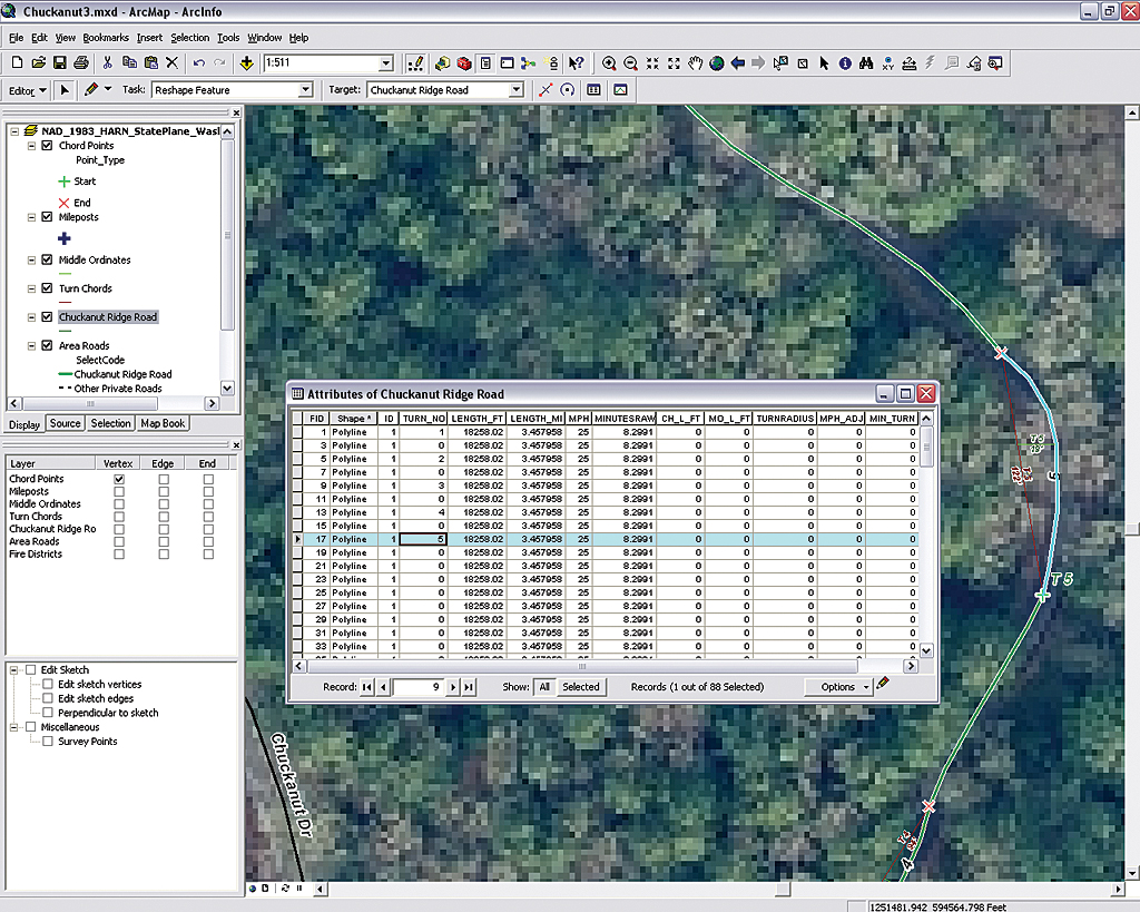
2. To begin, use the Edit tool to select the Chuckanut Ridge Road, which is one segment. Next, change to the Split Tool on the Editor Toolbar. Move the cursor to the endpoint of Turn Chord 1 and watch the cursor snap to the vertex.
3. Left-click once to split the line. Reselect the uphill (longest) portion of the road and grab the Split Tool again. Break the road at the start of T2. Continue this process in an uphill progression. This makes fixing numbering errors easier. When finished splitting the road, save these edits.
4. The next step is numbering the curve segments to match the Turn numbers. This is a manual process. Open the Chuckanut Ridge Road attribute table. On the map, select the turn segment for Turn 1 and enter 1 in the highlighted record in the TURN_NO field. Proceed to select and number turns from Turn 1 through Turn 47 and do not miss any curves.

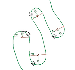Use an expression to label the radius of the turns.

5. When finished, sort data by [TURN_NO] and verify curves 1 through 47. Now, use Calculate Geometry to recalculate the length of all segments in both U.S. Feet and U.S. Miles. As an additional activity, recalculate raw travel times [MINUTESRAW] for all segments. Save the edits, end the edit session, and save the map.

Task 5: Joining Chord and Middle Ordinate Lengths and Calculating Turn Radii

Before calculating the radius of each turn, the Turn Chords and Middle Ordinates tables must be joined to the Chuckanut Ridge Road segments. Then the CH_L_FT and MO_L_FT fields in the Chuckanut Ridge Road table will be populated with values.

1. Open tables for Chuckanut Ridge Road, Turn Chords, and Middle Ordinates and adjust the size of each so all are visible.
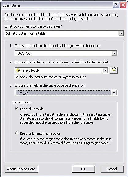
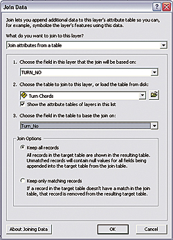
2. Right-click on the Chuckanut Ridge Road layer, choose Joins and Relates > Join and use TURN_NO as the field in this layer to base the join on, choose Turn Chords as the table to join to this layer and Turn_No as the field in the table to base the join on, and click on the radio button to keep all records.
3. Now calculate the length of all Turn Chords in the Chuckanut Ridge Road table. Use the Field Calculator to populate the Chuckanut_Ridge_Road.CH_L_FT field with the values from Chord1.Length_Ft. Then remove the join by choosing Joins and Relates > Remove Joins.
4. Next, join the Chuckanut Ridge Road table to the Middle Ordinates table. Right-click on the Chuckanut Ridge Road layer, choose Joins and Relates > Join and use TURN_NO as the field in this layer to base the join on, choose Middle Ordinates as the table to join to this layer, choose Turn_No as the field in the table to join on, and click on the radio button to keep all records.

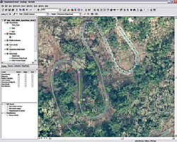
Applying Turn Radius, Ft.lyr thematically maps turns and shows the tightest turns with thick red lines.

5. Right-click on MO_L_FT and use the Field Calculator to populate the MO_L_FT field using values from MidOrd1.Length_Ft.
6. Now the radii of all 47 turns can be calculated. In the Chuckanut Ridge Road table, select all turns by attribute using the formula ([TURN_NO] > 0).
7. Right-click on TURNRADIUS and open the Field Calculator. Type (([CH_L_Ft]^2) / (8 * [MO_L_Ft])) + ([MO_L_Ft] /2) in the formula box. This is the algebraic form of the radius curve formula. Check to verify that all selected records calculate properly. Values will range from just under 25 feet to over 200 feet.
8. To label and study these turns, open the Properties dialog box for Chuckanut Ridge Road and select the Labels tab. Click the Expression button and type "T "& [TURN_NO] &VBNewLine & Round([TURNRADIUS],0) &"Ft" in the Expression box. Change the font to Arial 14 point and apply a halo. Click OK twice to apply the labels and make sure the Label Features box is checked. Inspect them to verify each turn number and radius. Turn the background image on and navigate back to CR MP 0.5 1:1,500.
9. To apply a thematic legend to these curves based on the turn radius, navigate to \Chuckanut \SHPFiles\WASP83NFH and load Turn Radius, Ft.lyr. Turn off the Chuckanut Ridge Road layer and check the turns. This Turn Radius, Ft.lyr uses the edited road file and applies a color legend that shows the tightest turns with thick red lines.
10. Inspect the map using the extent obtained with the MP 0.5 bookmark. Notice how all the switchback turns at approximately MP 0.7 have similar radii. This road was actually built by loggers nearly 100 years ago. Zoom out to the extent of bookmark CR All 1:15,000 to see the final product. Turn off any labels not needed at this scale. Save the map once more.

Acknowledgments

Special thanks to Skagit County GIS for sharing its excellent imagery and terrain data and to the Chuckanut Ridge Homeowners Association and Skagit Fire District 5 for the opportunity to develop and test this model. The author thanks the staff and students at Bellingham Technical College for their help in testing and refining this workflow and to Esri Canada Limited's Vancouver office for the chance to present this exercise to a sample audience.