ArcUser Online
|
:
|
In the July-September 1998 issue of ArcUser magazine, we learned how to import 1:100,000 scale USGS Digital Line Graph optional (DLG-O) format data into ArcView GIS by first converting it to Drawing Exchange Format (DXF) then using the CAD Reader extension to load DXF files. Once in ArcView GIS, we modeled boundaries, hydrography, hypsography, public lands, and transportation data sets; applied thematic legends to make the data more meaningful; and created an attractive two-dimensional map of the Bright Angel Creek and the Phantom Ranch area, near the center of Arizona's famous Grand Canyon. In this issue, we will make this two-dimensional map easier to read. Note the highlighted sections marked Version 3.1 Trick and ArcView 3D Analyst Trick that contain shortcuts and tips. First we will create more meaningful legend names by performing a table join with a dBASE file containing descriptive text. While still working in two dimensions, we will use the ArcView 3D Analyst extension to create a triangular irregular network (TIN) to add vertical relief to Bright Angel topography. After building a TIN, we will switch to three-dimensional mode and continue to model Grand Canyon terrain by draping two-dimensional line features onto the TIN. To test the model in three-dimensional space we will take a virtual rim-to-rim hike across the Grand Canyon. To practice the modeling described in this issue, you will need ArcView GIS Version 3.1 for all two-dimensional procedures and the ArcView 3D Analyst extension and a fairly powerful computer to create the TIN model and perform three-dimensional modeling. If you have not already constructed and saved the Bright Angel two-dimensional model described in the October-December 1998 issue, go to ArcUser Online at the Esri Web site (www.esri.com/arcuser) to get copies of previous articles that describe how to download and convert data and make the Bright Angel model. This article will show you how to enhance the Bright Angel model three-dimensionally. Using a Table Join to Build a Thematic Legend
When creating the model, we downloaded data from GC4 Tile 08 and renamed and converted six data sets. The DXF files should still be available in the project directory.
Look closely at the legends for hydrography, railroads, and roads themes. These themes were built by typing in specific
labels from a list provided in the last issue and are specific to data within Tile 08.
Now, using MAPLAYER.DBF, a dBASE table downloaded from the Esri Web site, we can create a legend that should work
for DLG-O data in all areas.
Turn off all themes except hydrography. With the hydrography theme visible and active, click the Open Theme Table button to display the attributes of the rivers and springs. The attributes used to create this thematic legend reside in the layer field and are not easily understood. The layer names loaded through the CAD Reader extension represent major/minor codes developed by professional cartographers. MAPLAYER.DBF will join these codes with more descriptive names. Joining Two Tables Go to the main Project window and select Tables. Verify that dBASE is the selected file type and that MAPLAYER.DBF is stored in your project directory. Use the Add button to add MAPLAYER.DBF in the model. This table contains over 500 records and its fields contain layer codes plus information about line color, style, and text descriptions.
A new, easily understood legend will appear. Select a color ramp for this legend using shades of blue. You can with individual colors and line thicknesses. Several data types, such as wells and springs, are truly point data and are not converted correctly. We are working on ways to correct this. Reopen the MAPLAYER.DBF table and repeat the above procedure to join MAPLAYER to the railroads and roads tables. Create thematic legends for these data sets also. You do not need to add MAPLAYER again since it should be available when you return to Tables in the main Project window. In the previous article, hypsography was mapped using elevation as a classification field and graduated color as a legend type. If you like this color scheme, do not change a thing. The boundaries and public lands data sets do not convert and load as consistently as other data sets such as hydrography or hypsography. If you experiment with table joins using these data sets don't get too frustrated. They are probably mapped using a unique value legend type. You may notice that many records contain the original DXF file name as a layer code. As we find consistent ways to handle these data sets, we will publish them. Save your project and get ready for t hree-dimensional fun! Creating a Topography TIN with ArcView 3D Analyst After remapping several data types using a table join, the ArcView 3D Analyst extension can be used to generate a really neat three-dimensional model. The first step in three-dimensional modeling creates a TIN to support data that does not contain built-in elevation information. Follow these steps to build the TIN.
A mass points process will break the topographic contour lines into many short vector segments. Endpoints of the vectors will build into vertices of triangles spanning between adjacent contour lines. Since each triangle's vertices will have several elevations, the triangle will display slope and aspect in three-dimensional space. Make the TIN the last theme in your legend so two-dimensional line data will be visible. With the TIN active, choose Theme then Properties from the menu. Note the number of triangles in this TIN. Due to its complex topography, this Grand Canyon TIN contains a large number of triangles. Triangle counts over 300,000 render slowly and can be hard to manage. This is where having a computer with a fast processor and enhanced graphic card pays off!
Click the legend box to activate the TIN and watch it grow before your eyes! A hill shade pattern with the sun low in the
northeast is applied. Turn on the other line theme--boundaries, hydrology, public lands, railroads, and roads. Inspect
your model to make any changes in the legends or color ramps of each theme. Changes made while working in two
dimensions are more quickly accomplished. Draping and Modeling Two-Dimensional Data in a Three-Dimensional World Now the real fun begins, but be patient. First, open a new three-dimensional view by returning to the main Project window and selecting 3D Scenes, located at the bottom just below Scripts. Rearrange your workspace by placing the 3D legend window in the upper left corner and expand the three-dimensional view to cover most of the remaining screen. Notice the three-dimensional display area and the three-dimensional Legend are represented as two separate objects on your desktop. The three-dimensional display takes over the desktop and can be closed or pushed to the bottom of the screen. It cannot be minimized like a two-dimensional view. Study the menu selection for 3D Scene Properties. Set the Map Units to meters. Just for fun, change the background color from black to sky blue and set the Sun Azimuth to southeast. Leave the Sun Altitude and Vertical Exaggeration factor unchanged for now. Return to your two-dimensional view. Select only the TIN and if it is visible, turn it off. Use Edit Copy Themes to copy the nonvisible TIN to the Theme Clipboard. Make the 3D Scene active and paste the TIN into the Legend window. After pasting the TIN, turn it on and wait patiently (possibly several minutes) as it loads and renders. This operation tests the computing and graphics performance of your computer. If your system chokes at this point, it may be necessary to build a smaller TIN by clipping out a small portion of the topographic contour lines. If the model renders properly, experiment with navigating, panning, and zooming through the model. Use the left mouse button to navigate, the right button to zoom, and the center button (or on two-button mice, left and right buttons together) to pan. If you are not familiar with these procedures, you may want to practice on a smaller, more easily managed model. In any case, be patient. This is a large model! Next, turn off the 3D TIN and save your project with the TIN off. Return to the two-dimensional view and select the hydrography theme. Turn the hydrography theme off and copy it to Theme Clipboard. Switch back to the 3D Scene and paste hydrography into the Legend window. Turn the hydrography theme on. Make it the only active theme and use the Zoom to Active Theme(s) button. Now, use navigate, pan, and zoom to explore the streams. Don't be too disappointed if they look flat. This theme has not been assigned to any base height source. We will fix that next.
After the streams redraw, move to the active theme and navigate through it. The hydrography lines are now draped on the TIN, positioned 15 meters above average height of the triangles in the TIN for visibility. Save your project again, then turn on the TIN. If all goes well, you will have an amazing Grand Canyon model in your 3D Scene!
To load other line themes from the two-dimensional view, turn the TIN off and return to the two-dimensional view.
Copy the boundaries, public lands, railroads, and roads themes to the Theme Clipboard. Move to the 3D Scene and
paste this group of themes. Choose Theme then 3D Properties and follow the procedure above to drape each theme.
Set these themes 15 to 25 meters above the TIN theme. Turn these themes on individually and in groups. If everything
looks reasonable, save your project. Navigate to a neat looking spot in the view, turn on the TIN, and wait. Navigation
through a large model is done most effectively with the TIN turned off. Now it's time to step back and really admire this three-dimensional model of Bright Angel! As with the two-dimensional model, you can observe relationships between hiking trails and canyons. Visually estimate the steepness of drainages. Imagine the elevation differences between the Colorado River and the canyon rims. Compare calculations made with the two-dimensional model to this model. Trace the Bright Angel trail as it follows the Bright Angel Fault across the Grand Canyon. Now you know why pioneers often followed fault zones when building a trail. Summary The three steps presented in this article have taught you how to enhance a DLG-based, two-dimensional model using ArcView GIS and how to create a complex three-dimensional terrain model with ArcView 3D Analyst. Now that you are a master Grand Canyon modeler, download data for other favorite areas from the USGS Earth Resources Observation Systems (EROS) site and build your own models. We are working on procedures for converting and mapping the newer USGS Spatial Data Transfer Standard (SDTS) format line sets and are reviewing methods to combine TIN, grid, and vector data into complex terrain models. Of course, we will also investigate inconsistencies and problems that arise from data development and modeling procedures. Stay tuned for future activities! Visit ArcUser Online at the Esri Web site to obtain copies of the articles in this series. These modeling methods will be taught at selected sites to be announced on the Esri mining solutions Web page. |
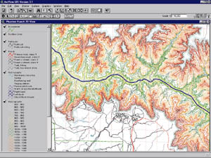 Start an ArcView GIS session and load the Bright Angel project. If you have a paper copy of the Grand Canyon East
1:100,000-scale quadrangle, you can use the map to refresh your memory of the data and to help you build a properly
coded model. In the menu bar, go to File, then Extension to load the CAD Reader and ArcView 3D Analyst extensions.
Open a two-dimensional view and verify that all data sets have loaded properly. Your model should look similar to screen shown.
Start an ArcView GIS session and load the Bright Angel project. If you have a paper copy of the Grand Canyon East
1:100,000-scale quadrangle, you can use the map to refresh your memory of the data and to help you build a properly
coded model. In the menu bar, go to File, then Extension to load the CAD Reader and ArcView 3D Analyst extensions.
Open a two-dimensional view and verify that all data sets have loaded properly. Your model should look similar to screen shown.

 A large TIN may take a while to build. The status line at the bottom of the screen will let you know how things are going.
After the TIN is built it will load into the current view, at the top of the legend window, with a topographic color ramp built.
The TIN data type is similar to a polygonal type.
A large TIN may take a while to build. The status line at the bottom of the screen will let you know how things are going.
After the TIN is built it will load into the current view, at the top of the legend window, with a topographic color ramp built.
The TIN data type is similar to a polygonal type.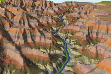 Your two-dimensional model could look similar to the screen capture shown here.
Save your project and close all other unnecessary programs before moving on to three-dimensional modeling.
Your two-dimensional model could look similar to the screen capture shown here.
Save your project and close all other unnecessary programs before moving on to three-dimensional modeling. Your completed model might look similar the
screen capture shown here.
Your completed model might look similar the
screen capture shown here.