ArcUser Online

Sample Size Matters
Caveats for users of ACS tabulations
By Lynn Wombold, Esri Chief Demographer

Once upon a time, counties were considered small areas. Today, households are literally the lowest common denominator. Increasing resolution has characterized data development over the past 30 years. We have traveled from states and counties down to blocks, nine-digit ZIP Codes, and even households by following the road paved by the Census Bureau's development of small area data and mapping. Our immediate future brings us to a crossroad where spatial analysis may continue to promote the study of small areas, but the census data that users have long associated with small area profiles will not support that analysis.

The American Community Survey (ACS) replaces the traditional sample data collected during the decennial census. Although the ACS covers the same subjects as the census sample, the method of collecting the data is very different, which produces real differences in the results. [An article in the October–December issue of ArcUser, "Changes and Challenges—Understanding American Community Survey Data," provides a more detailed comparison of ACS and Census 2000 samples.] Both the ACS and the census sample begin data collection with samples drawn from the Master Address File (MAF), but the sampling rates differ. The Census 2000 sample represented approximately 1-in-6 housing unit addresses at one point in time, April 1, 2000. The ACS represents approximately 1-in-40 addresses and a period estimate of population and housing characteristics compiled from monthly surveys.

Since full implementation of the ACS in 2005, the Census Bureau has been conducting monthly surveys of about 250,000 addresses with a goal of 3 million addresses surveyed annually. The ACS design oversamples small areas (similar to the census) and areas with lower mail response rates (unlike the census). The Census Bureau believes that these sampling rates will provide estimates that are approximately the same quality as the Census 2000 sample by using multiyear averages (three to five years) for smaller areas.

However, a cumulative survey base of 3 million represents 2.5 percent in one year, and 12.5 percent or 1-in-8 addresses over five years—compared to the average sampling rate of 1-in-6 or 17 percent from the Census 2000 long form. The ACS oversampling rate of 1-in-10 for areas with fewer than 200 addresses compares to the census sampling rate of 1-in-2 for areas with fewer than 800 addresses. Although both surveys draw samples from the MAF, the size estimates for the census long form sample were based on housing unit counts multiplied by occupancy rates from the 1990 census. This extra step qualified more small areas—especially areas with high seasonal populations—for oversampling.

At the county level, Census 2000 sampling rates actually range from a high of 50 percent in two counties to a low of 9 percent in one county due to the variation in size among sampling areas within the county. The average sampling rate for all counties was 23.6 percent, closer to 1-in-4 than 1-in-6. Looking at the counties by population size, Figure 1 displays the average sampling rate for the counties from the Census 2000 long form. The population size ranges represent the parameters set by the Census Bureau to report ACS data reliably: areas with 65,000 or more people (one year); areas with 20,000 to 65,000 people (three years); and areas with a population under 20,000 (five years).

The size of the sample in Census 2000 was selected to produce reliable estimates for small areas. Given the differences in the sampling rates, is five years sufficient to produce a sampling ratio as reliable as the Census 2000 sample? Figure 2 displays the average number of years necessary to achieve the sample size of the census long form, using sampling rates from 2.5 percent to 10 percent.

For the smallest counties (those with populations under 20,000), at the rate of 2.5 percent annually, it would take an average of 12 years to accrue the same sample base as Census 2000. Even the largest counties would need an average of 6.2 years to achieve the Census 2000 sample base at 2.5 percent annually. The sampling rate must be more than 5 percent to accumulate a sample base that is comparable to the Census 2000 sample in less than five years. Looking at the information displayed in Figure 2, counties with the largest sampling rates in 2000 (Maximum) would need more time. The larger (20,000+) counties with the smallest sampling rates in 2000 (Minimum) would still require three or four years at a sampling rate of 2.5 percent.

Unfortunately, few areas show a final sampling ratio of 2.5 percent. Since full implementation of the ACS began in 2005, the initial addresses selected for the samples total fewer than 2.9 million annually, only 2.3 percent of housing units. That ratio decreases dramatically after commercial or nonexistent addresses are removed and noninterviews are subtracted. Final interviews, including occupied and vacant housing units, correspond to about 1.6 percent of housing units. At the state level, the final interviews range from a low of 1.2 percent (Florida) to a high of 2.7 percent (North Dakota) of total housing units. Only three states have a final interview rate more than 2.5 percent—Minnesota, North Dakota, and Vermont.

Figure 3: Average household size estimates by the Census Bureau compared to forecasted values based on the change from 1980 to 1990

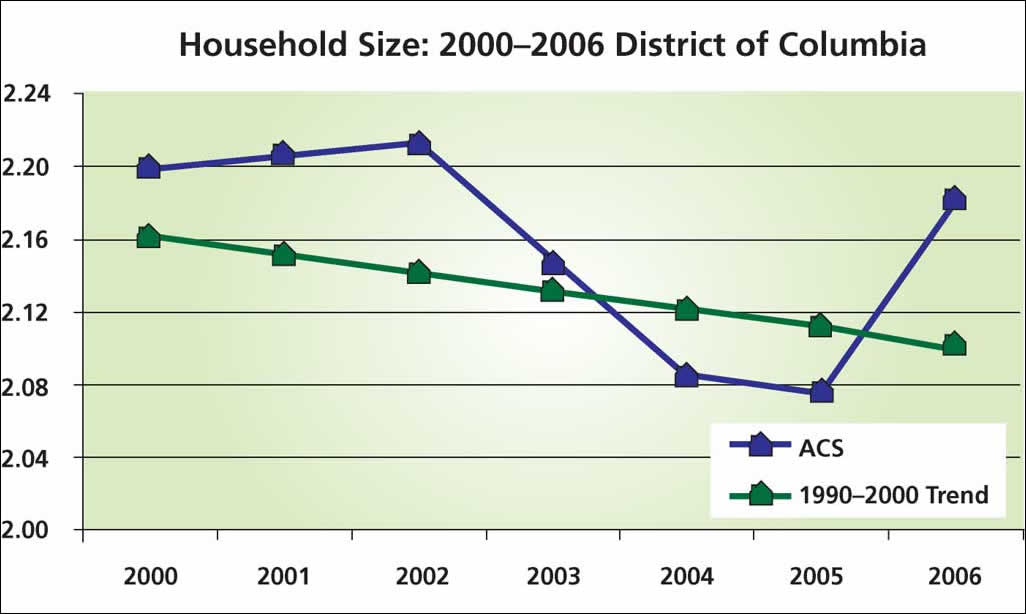
Without an increase in the sampling rate, estimates from the ACS will have larger standard errors, larger confidence intervals, and less reliability than the sample data collected from Census 2000. What does this mean to the data user? The accompanying graphs demonstrate the variability of the survey's estimates with one of the most stable demographic measures, persons per household or average household size. The relationship between the population in households and the total number of households incorporates both population characteristics (age, race and ethnicity, and marital status) and household composition (family, single person, or single parents) and is not subject to erratic changes in value. This stability enables smooth, relatively accurate forecasts of average household size, as shown in Figure 3. The extrapolation of a past trend line, 1980–1990, provides a relatively accurate depiction of the change in household size for the District of Columbia through the 1990s.

Using the same technique with a more recent trend line, 1990–2000, the extrapolated change in household size is compared to ACS estimates of household size, 2000–2006, in Figure 4.

Figure 4: ACS household size estimates compared to values based on the change from 1990 to 2000

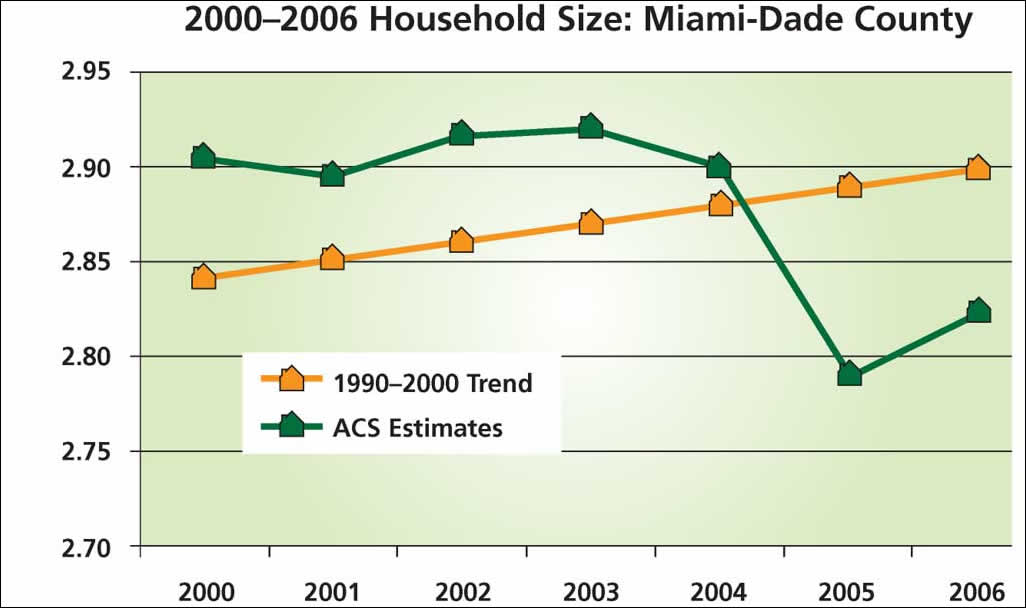
The change in ACS estimates is clearly more erratic than the expected change in household size. Add to this the fact that household population and housing units are weighted by independent estimates, and the variability is more difficult to understand. The District of Columbia is also the equivalent of a state. What happens in smaller states—or smaller areas such as counties? Figure 5 illustrates the same information for Miami-Dade County, Florida.

The ACS estimates of household size for Miami-Dade County are more variable than the estimates for the District of Columbia. Although Miami-Dade County is certainly smaller than the District of Columbia, it has a population base of about 2.5 million. The average population of counties with at least 65,000 people (the threshold for one-year ACS data) is much smaller—321,000. The average population size of all other counties is 21,700. Counties with a population less than 20,000 (which requires a five-year estimate of ACS data) represent more than 40 percent of all counties. Given the apparent volatility of estimates for areas with a population base measured in millions, will a five-year average be sufficient for the smallest counties, tracts, or even block groups?

Figure 5: ACS household size estimates compared to values based on the change from 1990 to 2000

Until 2008, even three-year period estimates will not be available for all eligible areas. The five-year period estimates are scheduled for 2010. However, an assessment of the ACS by the Committee on National Statistics concludes that areas with fewer than 50,000 people can expect "extremely imprecise" data. It has recommended combining not only tracts but also block groups and special tabulations, with eight- to ten-year averages to get "reasonably precise" estimates.

One thing is certain now: To use data from the ACS, it will be necessary to incorporate estimates of sampling error. Without the standard error estimates or margin of error (MOE) included with all ACS tabulations, it will be impossible to distinguish change from sampling error. Questions from readers are welcome and can be sent to the author at lwombold@esri.com.

About the Author

Lynn Wombold, chief demographer at Esri manages data development for Esri including the processing of census data and the development of unique databases such as the demographic forecasts, consumer spending, Retail MarketPlace, and Community Tapestry market segmentation system as well as the acquisition and integration of third-party data. She is also responsible for custom analysis and modeling projects. With more than 31 years of experience, her areas of expertise include population estimates and projections, state and local demography, census data, survey research, and consumer data. Prior to joining Esri, she worked for CACI Marketing Systems and was the senior demographer at the University of New Mexico. Wombold holds degrees in sociology, with a specialty in demographic studies from Bowling Green State University in Ohio. She has received CACI's Eagle Award for Technical Excellence and Encore Achievers. The author of numerous articles for industry publications, she frequently presents papers on demography.

Resources

National Research Council (2007). Using the American Community Survey: Benefits and Challenges. Panel on the Functionality and Usability of Data from the American Community Survey, Constance F. Citro and Graham Kelton, Editors. Washington, D.C.: The National Academies Press. [A free executive summary of this report is available online at www.nap.edu/catalog.php?record_id=11901. This document may be read at no charge.]