Interactive Site Suitability Modeling
A better method of understanding the effects of input data
By Clio Andris
Summary
Suitability modeling using raster data was one of the first—and remains a classic—GIS applications. The author proposes an interactive model that addresses one of the shortcomings of this approach to suitability modeling. The author's approach relies on vector data and uses tools in the ArcGIS Spatial Analyst extension. It automates processing by using the Field Calculator and ModelBuilder.
In suitability modeling, spatial data is classified and combined to identify sites most suitable for a specific use. Factors are given numerical values that indicate if their presence is detrimental or conducive to the desired use.
 |
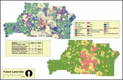
| Land-use data is reclassified from a nominal classification, such as High Density Residential, Industrial, Cemetery, or Park, to the index classification of 0-2-4. In this classification, land-use areas conducive to use as an airport are assigned a value of 4. |
This article addresses a shortcoming of a popular method for modeling suitability using rasters. After input rasters have been processed (cells are multiplied, added, etc.), the final raster shows resulting cell values from raster calculations. However, this final raster does not show the cell values of the input rasters. In the classic suitability raster, one could wrongly assume that if two different cells each have a score of 12, their input layers are similar. This is misleading because the factor values that contributed to this score of 12 could be completely opposite as shown in the accompanying table.
Weighting certain factors positively or negatively to influence the final suitability score is one way to account for the contribution of an individual layer to the final model. For example, if slope greatly affects a site's suitability, this factor can be accounted for through the cell values assigned to slope. However, it would be beneficial to see which factors feed into a certain cell value. Creating an interactive model provides information about the cell values of all input features and the final suitability raster. In addition, the challenge of visualizing more than one value per cell is addressed by this model through using the Identify tool to show input and output cell values on-click. Incorporating this functionality makes the new model interactive.
The premise for this site suitability model was developed by THE LPA GROUP INCORPORATED as part of a project for siting a potential general aviation replacement airport. In considering potential sites, the civil engineering firm took into account factors such as environmental constraints and impacts, aeronautical requirements, topography, accessibility/suitability, utilities, consistency with city/county planning, cost of developing the site, and proximity to the population served.
 |
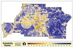
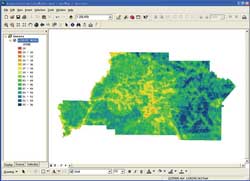
| In the output grid, suitable places for an airport are indicated by higher numbers in dark blue. |
Land use was reclassified using values of 0, 2, and 4. A value of 4 represented the most suitable area and a score of 0 was assigned to high-density residential and urban spaces because they were not suitable for airports. The layers were added to produce the final model. In this model, cells' final values range from 28 to 58. Higher values indicate land more suitable for the airport.
| Cell 1 | Cell 2 |
| Layer | Score | Layer | Score |
| Highways | 4 | Highways | 0 |
| Railroad | 4 | Railroad | 0 |
| Elevation | 4 | Elevation | 0 |
| Landfills | 0 | Landfills | 4 |
| Airports | 0 | Airports | 4 |
| PopDensity | 0 | PopDensity | 4 |
| Suitability | 12 | Suitability | 12 |
Cells with different land feature values can seem identical in a suitability raster.
Preparing Input Data for an Interactive Model
 |
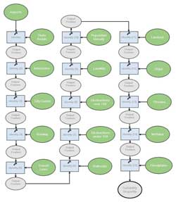
| An example of a model that uses the Identity tool and input shapefiles |
An overview of the process of creating an interactive site suitability model follows. Unlike the raster method, data is kept in vector format for this model. Often, some data processing operations, such as slope calculation or distance to feature, require raster data input. For data in raster format, use the GridShape tool available through the Raster Calculator in the ArcGIS Spatial Analyst extension. [Search on GridShape in ArcGIS Desktop help to locate the tool's syntax.] In developing a feature classification system, the range of numerical values indicated factors that contributed to suitable sites.
- Open the shapefile attribute table and add a new field. Clearly label the field with the name of the factor being considered. In this example, because proximity to railroads is being considered, the new field will be labeled RAIL.
- Use the Select by Attribute tool to select records that contain field values that correspond to the same classification value. For example, if a two- to five-mile proximity to railroads is preferred, select those records so they can be assigned a value of 4.
- In the attribute table, click Show: Selected. Right-click on the RAIL field header and select Field Calculator. In the Field Calculation Workbox, type the classification value (in this case, 4) to populate the RAIL field of the selected records. Now click Show: All table view and note that some records now hold the value 4 for attribute field RAIL.
- Repeat this process with the remaining records in the shapefile until each polygon has a classification value assigned for the RAIL field in the attribute table. Once this layer is complete, the process is repeated for other input layers.
- If raster reclassification is easier for multiple index values, this goal could be more rapidly accomplished by reclassifying each raster using the Reclassify tool in the Spatial Analyst extension toolbar, then converting the output raster to shapefile based on the preferred field (i.e., use the WEED option for the GridShape tool).
- For each input shapefile, isolate the input field by deleting all attribute fields (except the FID and Shape fields, which are required) other than the new field. For the proximity to rail shapefile, the FID, Shape, and RAIL fields are retained in the attribute table.
Use ModelBuilder to Fuse Input Datasets
After creating input shapefiles for the factors being considered, ModelBuilder can be used to automate the production of the final suitability shapefile.
- In ArcToolbox, create a new toolbox by right-clicking on an empty portion of the ArcToolbox pane and choosing New toolbox. Right-click on the new toolbox and choose New > Model.
- In ModelBuilder, drag and drop the first two input layers created previously into the ModelBuilder workspace. In the example shown in the accompanying illustrations, the Airports and State Roads layers were added first.
- Next, add the Identity tool from ArcToolbox by choosing Analysis Tools > Overlay > Identity and connecting the first and second layers to it.
- Add another Identity tool, and connect it to the previous output feature and a new layer.
- Repeat for each input layer. The final output will be the suitability shapefile.
Calculate Suitability Score
 |
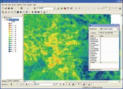
| An interactive suitability model with the Identify tool window |
From the suitability shapefile generated by the model, the suitability score can be calculated. Add a new field called Score or Index to the attribute table for the suitability shapefile. Right-click on the field name to open the Field Calculator. The Field Calculation Workbox in the Field Calculator dialog box will take the same expression that would be used in the Raster Calculator for the classic raster-based method for evaluating suitability. If the model's score is compiled by multiplication, multiply each attribute (e.g., [RUNWAY] * [LANDFILL] * [RAIL]). If the model's score is calculated by adding each layer, then use an expression, such as [RUNWAY] + [LANDFILL] + [RAIL], including all attributes in the equation. Note that number and names of attributes should equal the number and names of input layers. This process results in one single shapefile with all input information. For best visualization, symbolize each polygon in the output shapefile without outlines.
Summary
This method evokes the concepts of Integrated Terrain Units Mapping, described by Jack Dangermond and Eric Harnden in "Map Data Standardization—A Methodology for Integrating Thematic Cartographic Data Before Automation" that appeared in the Spring 1990 issue of ArcNews. This approach, in vogue in the 1980s, also generated a single set of features that were amenable to SQL queries and summation. In addition, this method eliminates the need for multiple rasters or shapefiles and the burden of turning layers off and on to overlap data from input layers with the final model.
 |
| Final map of airport suitability factors |
The information gain is strengthened because the user interacts with the model by using the Identify tool. The information on the Identify tool dialog box can be manipulated by right-clicking to sort or hide fields. This method allows the user to understand why an area has a certain suitability score and the factors that contributed to a high or low score.
One limitation of this method is that resulting polygons can take on sharp, shardlike shapes. In a raster model, the cell size can be a normalizing factor. Cells can be quantified and uniformly converted from cell count to area. In the interactive model, unusual shapes make areas more difficult to compare.
However the interactive model avoids some problems of a raster model. Areas with the same characteristics are treated as one polygon. This model does not require a user-defined cell size. Also, diagonal features are not lost or compromised by the vector-to-raster conversion. For easy dissemination of the results of this method, the interactive raster can be published in ArcReader with directions to use the Identify tool.
For more information, contact Clio Andris, University of South Carolina, at clio@sc.edu or 803-777-1282.
About the Author
Clio Andris is currently pursuing a master's degree in geography from the University of South Carolina with an emphasis on GIS and computer science techniques. She interned in the Environmental Planning Department at THE LPA GROUP INCORPORATED in Columbia, South Carolina. At LPA, she worked with GIS analyst David Grigg and Jim Duguay, manager of aviation planning. Headquartered in Columbia, South Carolina, LPA provides complete planning, environmental, design, and construction services for airport, highway, bridge, and architectural development programs.
|
