Crafting Better Decisions
Creating a link between belief networks and GIS
By Jeff Hicks and Todd Pierce, University of North Carolina, Asheville's National Environmental Modeling and Analysis Center

This article as a PDF .

Considerable research has led to an increased understanding of how human activity influences the landscape and has provided more options for managing forests in an ecologically sound manner. With advances in GIS technology, decision-making techniques, and environmental protection policies, more effective and integrated management approaches are available.

The Comparative Risk Assessment Framework and Tools (CRAFT), one such approach, has been developed by the U.S. Forest Service's Eastern Forest Environmental Threat Assessment Center (EFETAC) to improve the quality of decisions for forest and natural resource managers. CRAFT is designed to help planning teams focus on the most important issues, organize their analyses, and use the right tools and data in a facilitated environment. CRAFT has four phases:

• Specifying objectives: What's the problem?
• Designing alternatives: What to do?
• Modeling effects: What could happen?
• Synthesis: What to communicate?

To better model the effects of different alternatives, CRAFT uses belief networks [also known as Bayesian networks, Bayes networks, or causal probabilistic networks] and influence diagrams to model uncertainty about the world by combining both common sense and observational evidence based on the theory of Bayesian statistics.

Essentially, a belief network includes a series of variables that represents real-world attributes and each variable has several states. For example, a variable could be whether a lamp shines and its states could be true or false. An expert on those attributes connects the variables in a graphic network that shows how one or more variables cause a change in another variable (Figure 1).

Figure 1: A simple network that predicts the outcome of a light working based on real-world observations

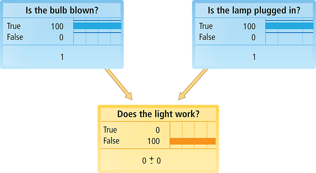
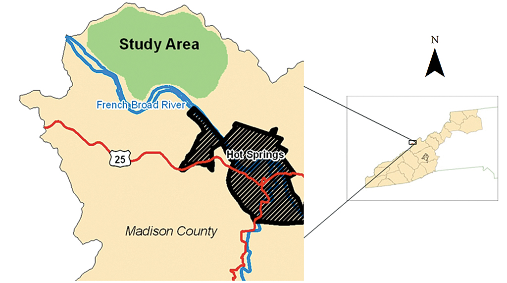
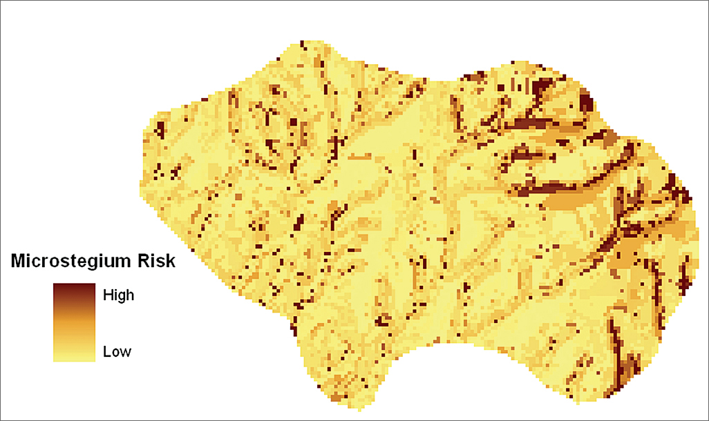
The primary feature of a belief network is its ability to "learn" and continually refine the extent of a relationship between two variables by using conditional probabilities. Instead of making educated guesses between two factors, a user (or in the case of CRAFT, a group of users) can create a network, make observations on those variables, and compile the findings as cases. It is from these cases that the belief network software determines the conditional probabilities between two variables.

While the theory underlying Bayesian statistics is complex, a software package commonly used for belief network modeling—Norsys Netica—is approachable, graphic, and intuitive. In addition, outputs are not as intimidating as the results generated by many statistical packages.

Belief networks are useful for CRAFT and other risk assessment tools but have not been linked to GIS so variables can be placed in a spatial context. Although some networks, such as ones used to determine a likely disease diagnosis for a given set of symptoms, do not have an appropriate spatial context, for other networks, such as models used to determine likely forest health given a set of threats, spatial context is critical. This information can answer questions like, What areas of forests are most at risk? and Where can mitigation efforts be prioritized to leverage limited resources?

Researchers at the University of North Carolina at Asheville's National Environmental Modeling and Analysis Center (NEMAC) looked for current solutions to tie belief network models to a GIS that would support the use of CRAFT but couldn't find anything that allowed for in-depth risk analysis or had a suitably generic process. It was critical that the process be general enough to apply to any spatial risk assessment from invasive species to wildfires to landslides. Consequently, NEMAC decided to write its own tool using the ArcGIS Desktop application ArcMap and incorporating Python scripts and Netica, a program for working with Baysian belief networks from Norsys Software Corp.

As a test case to develop the method, NEMAC investigated the risk that an invasive species known as Japanese stilt grass, or Microstegium vimineum (MIVI), would encroach on an area near Hot Springs in the Pisgah National Forest in North Carolina. Invasive species data was collected by Equinox Environmental (equinoxenvironmental.com), a consulting and design firm.

Figure 2: Location map for the study

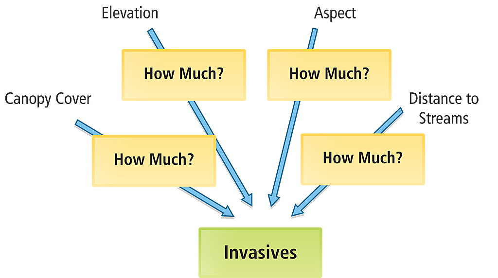
Within the study area (see Figure 2), Equinox Environmental collected GPS survey paths and marked every MIVI occurrence as a point feature. The paths were locations where MIVI was known to be absent and the points were locations where MIVI was known to be present. With the proposed process, this information could then be used to assess the risk of MIVI occurring in the rest of the study area that had not been surveyed. Simply put, the absence of evidence was not evidence of absence.

First, a conceptual model (Figure 3) was created in consultation with scientists from EFETAC. [EFETAC, established by the U.S. Forest Service, uses an interdisciplinary approach in developing new technology and tools that anticipate and respond to threats to eastern forests.] While tracking the factors associated with the location of invasive species is incredibly complex, NEMAC simply sought to test a method for putting geographic information into a Bayesian statistical context and returning the results to geographic space. As a result, the location variables used were based on a trusted data source, The National Map Seamless Server, a data resource provided by the U.S. Geological Survey that is publicly available and easily accessed.

Figure 3: A basic conceptual model showing factors that lead to the occurrence of invasive species. The yellow boxes ask, What is the extent to which each of these factors contributes to suitable locations for invasive species?

The process for preparing data in ArcMap, exporting data to Netica, performing analysis in Netica, and importing the results back into ArcMap is summarized in the following five stages.

Stage 1: Location Data Preparation

1. Obtain elevation, streamline, and canopy cover data from The National Map.
2. Derive aspect from elevation.
3. Create a multiple ring buffer around streams and convert the vector layer to raster.
4. Prepare location data so all rasters have the same projection and resolution and that each raster cell snaps to the same grid.
5. Reclassify all data to appropriate classes. Reclassification was an iterative process. (Initially, aspect data was classified equally based on the four cardinal directions. However, an EFETAC scientist pointed out that one class for north (270��90�) and three equal classes for southeast, south, and southwest, respectively, were more appropriate classifications.)
6. Clip all data to study area boundaries.

Stage 2: Survey Data Preparation

1. Convert vector survey data to raster with the same snap grid as the location data.
2. Reclassify survey data into three classes: known MIVI absence, known MIVI presence, and unknown MIVI presence or absence (i.e., areas not surveyed).
3. Clip the MIVI presence/absence raster to the study area boundaries.

Figure 4: Representation of the data inputs overlaid with a screen capture from Netica. In this example, the user has selected hypothetical states for each variable and Netica has updated the probabilities for the presence/absence node.

Stage 3: Data Combination and Export

1. Use the Combine tool (Spatial Analyst Tools > Local > Combine) to create an aggregate raster. (The Combine tool visits every cell in the study area. For each cell, it records the value for the presence or absence raster and the values for all location rasters.)
2. Use a Python script written by NEMAC to export this dataset as a simple comma-delimited text data table where every cell in the study area is a single row and each variable—all location rasters and the presence/absence raster—has a unique column.

Stage 4: Export Data from ArcMap and Import It into Netica

1. Import the comma-delimited text file into Netica. Netica automatically creates one node for every column. Each node represents a single variable for all location rasters and the presence/absence raster.
2. Configure each node so its states correspond to the classification applied to the map in ArcMap. Note that the presence/absence raster has a value for unknown. A state should not be configured as unknown because this represents areas that were not surveyed. Statistics should be generated solely on areas that were surveyed. By not creating a state for unknown values in the presence/absence node, Netica skips all cases that represent areas that were not surveyed.
3. Arrange and connect the nodes to represent the conceptual model.
4. In Netica, select Incorporate Case File to go through the entire data file and record the observations for each row (i.e., every cell in the study area).
5. The case file populates a table in every node, including the presence/absence node, and determines probabilities based on these tables.

Figure 5: The first few lines of the presence/absence node table in the Netica network file. On the right, each node feeding into the presence/absence node has its own column. Each of its possible states is combined so that each row represents a unique combination of the variable states. On the left, the probabilities are represented for each state of the presence/absence node.

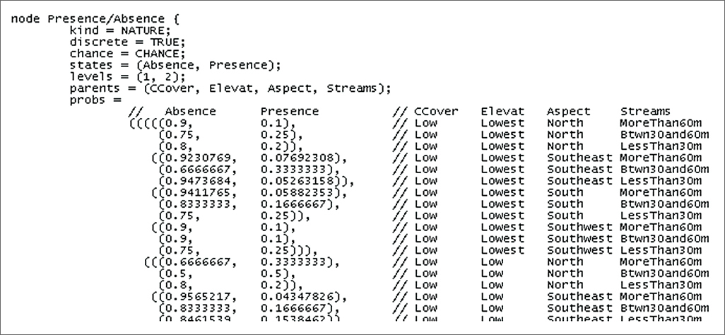
For example, the first row might represent a location where MIVI was present, had a moderate canopy cover, was at the highest elevation state, had a south aspect, and was more than 60 meters from a stream. Netica moves on to the next row where the conditions might have been different. After Netica goes through the entire study area, it calculates the probability of each state occurring in the presence/absence node given every possible combination of states in the location nodes. Netica can assert that for the stated combination described previously, there is a 16.7 percent chance that MIVI will occur in places with those conditions.

In Netica, users can interact with the network to model what-if scenarios. As a user clicks on different states in each node and sets them to 100 percent certainty, the probabilities represented in each other node (based on what is known so far) are updated and displayed. These hypothetical situations do not alter the probability tables. Rather, they show how other variables respond when one or more variables are set to certain states.

Stage 5: Export Data from Netica and Import It Back into ArcMap

Netica stores the conditional probability tables as a Netica network file that shows the probability of each state in the response node for every combination of node state combinations.

1. Parse the network file to a text table using another Python script written by NEMAC. Each presence/absence variable and each state of the location variables has its own column. Each row represents every combination of the states of the location variables and the corresponding probabilities for each state of the presence/absence variable. This script also adds a new column to the aggregate raster, created by the Combine tool, for the MIVI presence probability values.
2. The script then goes through each cell in the aggregate raster, matches the combination of states for each of its constituent variables to that same combination in the Netica output, and inserts the corresponding MIVI presence probability value into the column created in the previous step.

Figure 6: The output of the Python script in ArcMap: the risk map for MIVI presence

At this point, every cell of the survey raster has a probability for MIVI presence. When this field is symbolized and displayed, the result is a risk map for MIVI presence. Given the simplicity of the variables investigated, this risk map is probably not the most accurate assessment of where one might find MIVI. However, this method allowed NEMAC to successfully take geographic information, use Bayesian statistical analysis, and present the results in a geographic context.

NEMAC is working with EFETAC to refine the belief network-GIS link and use it in other studies and upcoming CRAFT projects. Most significantly, this process is not limited to invasive species risk. NEMAC is investigating other potential uses for the process to ensure its generality and is also working to simplify and automate the process, more tightly integrating ArcMap and Netica.

For more information, visit the NEMAC Web site (nemac.org) or contact the authors, Jeff Hicks at jhicks@unca.edu or Todd Pierce at tpierce@unca.edu.

Acknowledgment

The authors thank Dr. Danny Lee and Dr. Steve Norman at EFETAC and Karin Lichtenstein, Jim Fox, and Alex Krebs at NEMAC for their assistance and advice.

About the Authors

Jeff Hicks is a recent graduate of the University of North Carolina Asheville Environmental Studies program. With a varied background in multimedia and graphic design, he was drawn to GIS because it combined his interests in technology and the environment. He began his work on the belief network-GIS link as a student intern for NEMAC and has gone on to become geospatial analyst at NEMAC. Hicks currently is a key contributor to a collaborative effort with the U.S. Forest Service in the production of the Western North Carolina Report Card on Sustainability. He also assists with research on creative ways of integrating geographic data in visualization environments.

Dr. Todd Pierce has worked in GIS for more than 18 years and has specialized in GIS and Web programming for 12 of those years. He holds a B.S.E. degree in electrical engineering from Tulane University and a doctorate in geography from Oxford University in the United Kingdom. He is responsible for linking GIS and databases to the Web at NEMAC, where he leads the development of an online multihazard risk tool for mitigation planning. He also assists with development of geographic decision facilitation processes that use Web applications and data visualization techniques to support public policy decision makers with land-use planning; flood mitigation and response; forest preservation; and other community issues.