Storing data in multiple dimensions allows earth scientists and GIS analysts to capture and analyze data gathered from under the earth’s surface, from its atmosphere, and from its oceans.
GIS workflows have historically been two-dimensional. However, in addition to the familiar x and y spatial dimensions, multidimensional data can have one, and sometimes two, additional dimensions.
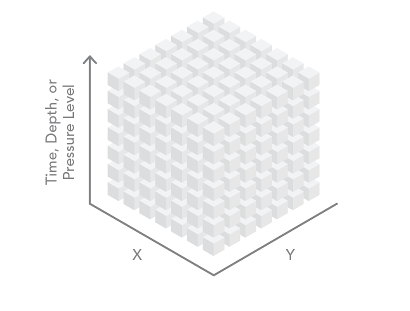
Three of these dimensions can be visualized as the axes of a cube. The data can be regularly gridded (as a raster) or in point format (with one point at the centroid of each cell in the array). For ocean data, the third dimension contains data on depth (x,y,z). For atmospheric data, the third dimension often contains data on the pressure level in a standard atmosphere (x,y,p). The third dimension is also used to store time (x,y,t).
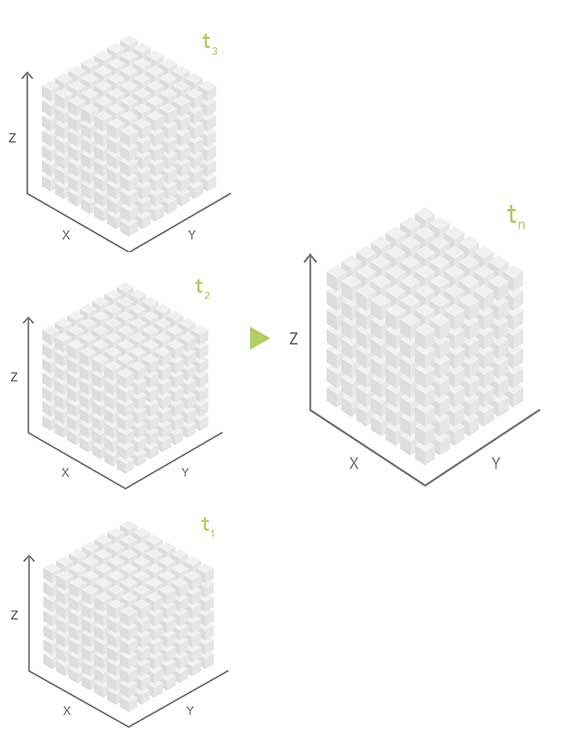
Four-dimensional datasets store spatial data (x and y dimensions) at various depths or altitudes (z) at different times (t), yielding an x,y,z,t dataset.
Unlike general relational database or GIS-based formats, scientific data formats are optimized for storing multidimensional scientific data and the associated metadata. To efficiently store multidimensional data, the science community has developed specialized file formats such as Network Common Data Form (netCDF), Hierarchical Data Format (HDF), and Gridded Binary (GRIB).
Support for netCDF was introduced in the ArcGIS platform in version 9.2 through the Multidimensional toolbox. Multidimensional tools support raster, feature (point), and tabular data. Support for raster data stored in HDF and GRIB was introduced through the mosaic dataset in version 10.3. ArcGIS support of these multidimensional formats enables the integration of scientific data into GIS workflows and allows ArcGIS to serve as a platform for scientific data management and analysis.
Analysis Patterns
According to Martin Fowler, analysis patterns are a way of documenting “an idea that has been useful in one practical context and will probably be useful in others.” Fowler, a British software developer who has specialized in object-oriented analysis and design, UML, patterns, and agile software development methodologies, introduced this concept in 1997 to provide a high-level abstraction of an analysis workflow. Slice by slice (within one file or in separate files), location by location, aggregation, and custom are the four main patterns for analyzing multidimensional data. The first three patterns can be accomplished using geoprocessing tools and ModelBuilder in ArcGIS. The last approach—custom—requires some programming.
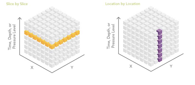
Slice by Slice
The slice-by-slice analysis pattern works with data in the same file or with data contained in separate files. A common multidimensional data workflow processes the dataset one slice at a time. That one slice can be one depth level, one altitude level, or one time period. Think of the multidimensional dataset as a stack of playing cards. Each card in the deck is peeled off as a two-dimensional slice, and it can be analyzed using some of the hundreds of geoprocessing tools available in ArcGIS. One disadvantage of this analysis approach is that it doesn’t include information from any other depth, altitude, or time slice.
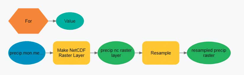
To begin slice-by-slice analysis, run one of the Make NetCDF tools from the Multidimension toolbox. This toolbox contains geoprocessing tools that create a netCDF raster layer, feature layer, or table view. Each of these tools has an optional parameter that allows the user to select the dimension (slice) that will be used to create the netCDF layer. The dimension value can be expressed as either a value (mm/dd/yyyy) or as an index.
The first-dimension value in a netCDF file has an index of zero. The dimension index is increased by one for each slice. For example, a netCDF file containing five time slices might have dimension values of 2001, 2002, 2003, 2004, and 2005. The same time slices could be referenced using the dimension indexes 0, 1, 2, 3, and 4.
When iterating through the slices of a netCDF file, it is often easier to use dimension indexes especially when using ModelBuilder with an iterator. The iterator starts with zero (the first slice of the netCDF file) and loops through the model until the last slice of the netCDF file is processed. The user must specify the end value of the iterator.
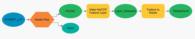
While netCDF files are designed to contain multiple slices of data, sometimes processing constraints, such as file size, rapid update cycles, or the need to move files quickly over the web, prohibit creating large netCDF files with many slices. This is often the case when netCDF files must pass through security firewalls or are the output of models that produce new time slices frequently.
To circumvent these constraints, data providers can create a new netCDF file for each slice. It is then the responsibility of the user to analyze these files one by one or aggregate them into a new file. The workflow to analyze the files one by one is very similar to the slice-by-slice method within a single file.
Location by Location
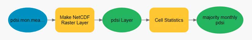
Raster-based multidimensional data can be thought of as a series of regularly spaced grids stacked on top of each other. Each slice in the stack represents a different depth, pressure level, or time. For some analyses, the analyst needs to process each raster cell (location) across depths or across time. Conceptually, this is like sticking a skewer through the cube at each location and performing some operation on all the cells the skewer touches. This workflow can be accomplished by stacking the slices of the multidimensional data into a multiband raster. Some geoprocessing tools, such as Cell Statistics and Band Collection Statistics, automatically know how to process multiband rasters.
Spatial and/or Temporal Aggregation of Point or Tabular Data
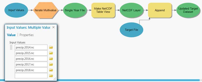
The multidimensional mosaic dataset is the preferred solution for spatially and temporally aggregating multidimensional raster data. However, geoprocessing-based workflows are required to aggregate feature or tabular data. File size, rapid update cycles, or other constraints often cause scientific data to be organized so that each year of data is in a separate file. A common pattern is to aggregate data into a single file and then perform analysis. An example could be creating monthly means for a number of years.
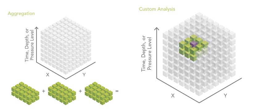
Custom Analysis Using Python
The Make NetCDF Raster Layer, Feature Layer, and Table View geoprocessing tools, along with the powerful capabilities of the multidimensional mosaic dataset, enable a wide range of workflows for analyzing multidimensional data. In some instances, however, the slice-by-slice or location-by-location approaches may not be sufficient. Fortunately, with the 10.3 release of ArcGIS, the new netCDF4 Python library began shipping as part of the ArcGIS platform.
The netCDF4 library allows you to easily inspect, read, aggregate, and write netCDF files. When data is read by the netCDF4 module, it is stored as a numPy array, allowing access to the powerful slicing syntax of numPy arrays. Data can be sliced by specifying indexes. For example, the variable tmin has three dimensions: year, latitude, and longitude. By specifying an index (or a range of indexes), the three-dimensional data cube can be sliced into a smaller cube.
Conclusion
The ArcGIS platform provides many ways to analyze the multidimensional scientific data, enabling modeling and greater understanding of earth phenomena. Esri continually develops and enhances tools and workflows for acquiring, managing, analyzing, visualizing, and sharing multidimensional data.
About the authors

Kevin A. Butler