In addition to expertise in GIS and data modeling, author Mike Price has extensive experience as a first responder and has been a volunteer fire fighter in Moab, Utah, for several decades. Approximately six years ago, he began experimenting with a multimodal response network, combining data on nearby trails and county roads into a single complex network. To predict travel times on various trail segments, he modeled slope using a US Geological Survey 10-meter digital elevation model and has field tested travel times by foot, bike, and motorized vehicle.
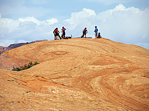
In the exercise scenario, an off-duty emergency medical technician (EMT) who is hiking on a mountain bike trail in Moab, Utah, encounters a cycling accident. A cyclist has taken a tumble and appears to have broken his collarbone and sustained abrasions but is conscious and coherent. The EMT calls 911, reports the victim’s location and condition, and awaits emergency personnel.
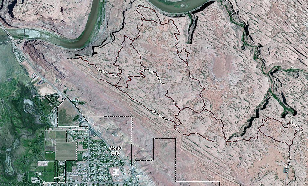
Response to this incident will require identification and routing of emergency medical and search and rescue (SAR) responders to their base facilities in and near Moab as quickly and efficiently as possible. The exercise describes how to create a multimodal network dataset to accomplish this. It ends with queuing these resources for deployment.
Preparing Data for a Multimodal Network
This portion of the exercise will consist of creating a Transportation geodatabase, building a new feature dataset, importing the transportation shapefiles into it, and calculating distance and time fields for those layers. To begin this exercise, download [ZIP] the Slickrock Rescue training set. Unzip it to a local drive.
1. Start ArcMap 10.1 and choose Customize > Extension to verify that a Network Analyst extension is available and active. Choose Customize > Toolbars to make the toolbar visible.
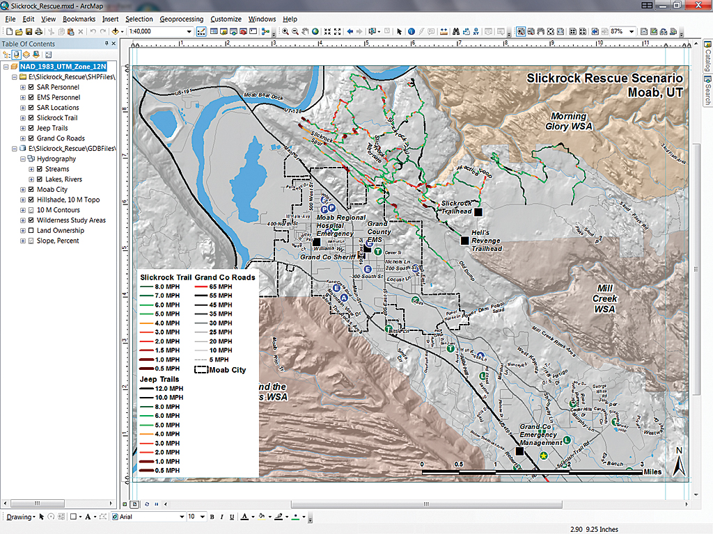
2. Open \Slickrock_Rescue\Slickrock_Rescue.mxd and inspect the data layers and their sources. Basemap data resides in a file geodatabase, and all transportation layers are shapefiles.
3. Close ArcMap and open ArcCatalog. Navigate to \Slickrock_Rescue_GDBFiles, right-click the UTM83Z12 folder, and create a new file geodatabase named GC_Transportation.
4. Right-click GC_Transportation and choose New > Feature Dataset. Name it SR_Response. Set the coordinate system to NAD 1983 UTM Zone 12N and accept the defaults for the rest of the parameters.
5. To import roads and trails into this feature dataset, right-click SR_Response and select Import > Import Feature Class (single). In the ArcCatalog window, select Slickrock Trail from the SHPFILE folder them to the Import wizard. To ensure that the entire shapefile is imported, click the Environments button at the bottom of the Import wizard and set the Processing Extent to Union of All. This is a very important step. Click OK. Repeat the process for Jeep Trails, and Grand Co Roads shapefiles.
6. After all transportation feature layers are imported, close ArcCatalog and open ArcMap. Create a new Group Layer in the TOC called SR_Response and drag the new layers to it.
7. To reuse thematic mapping that already exists for shapefiles, change the data pointer from each source shapefile in Transportation Group to its corresponding Feature Class in SR_Response. Begin by double-clicking Slickrock Trail to open its Properties, click the Source tab, and click the Set Data Source button. Choose Transportation_Group_Slickrock_Trail as the data source. Repeat this step for Jeep Trails and Grand Co Roads. Once this is done, remove the SR_Response group from the TOC and save the map.
8. Right-click the Slickrock Trails shapefile and open its attribute table. Notice that slope-adjusted speeds are already posted, but the segment distances in miles (MILES) and travel times in decimal minutes (MINUTES) are set to zero.
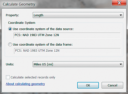
9. Right-click the MILES header and select Calculate Geometry. Calculate the Length in Miles US.
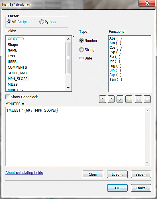
10. Once MILES are calculated, the travel time MINUTES for each segment can be calculated using its length and slope-adjusted speed. Right-click the MINUTES field header, open the Field Calculator, and use this formula:
MINUTES = MILES * (60 / MPH_SLOPE).
Carefully check the expression before clicking OK.
11. Perform the same operations on Jeep Trails. For Grand Co Roads, calculate length in miles for the MILES field. For the MINUTES field, use
MINUTES = MILES * (60 / SPEED_MPH)
as the expression.
12. Save the map and close ArcMap and reopen ArcCatalog. When creating and building a network dataset, data locks are often problematic. To avoid possible locks, create and build SR_Response in ArcCatalog with ArcMap closed.
Creating a Network Dataset in ArcCatalog
1. Open ArcCatalog and choose Customize > Extension and verify that a license for the Network Analyst extension is available and is active.
2. Navigate to Slickrock_Rescue\GDBFiles\UTM83Z12\ GC_Transportation\SR_Response and right-click the SR_Response dataset. Select New > Network Dataset. Click Next.
3. Accept the default name and specify a 10.1 network dataset. (Note that while 10.0 is an alternate version, 9.x is not.) Click Next and, in the next window, click the radio button next to Select all feature classes. Click Next.
4. Click Yes for Global Turns for all network participants and click Next. Click the Connectivity button and check the Connectivity Policy for network participant. They are designed to perform with endpoint connectivity, so verify that End Point has been specified. For some networks, Any Vertex might be considered, but these are very carefully constructed, and End Point is a very safe, stable choice. Click OK to close this window and click Next.
5. The Grand County roads and trails are quite simple, with no one-way streets or limited access, so this network will not use elevations to modify connectivity. Click the None button and click Next.
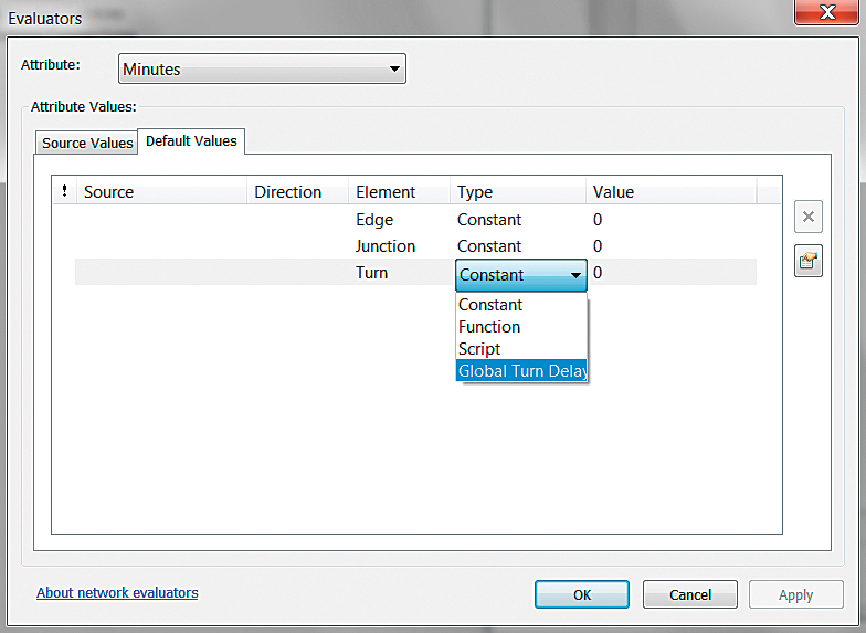
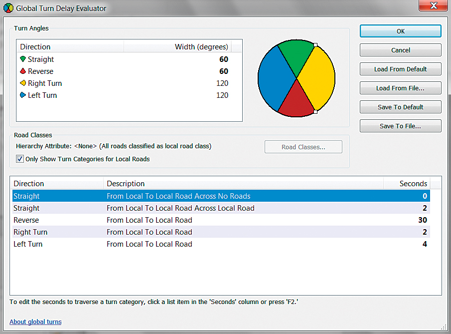
6. Now to add to the global turn rules. Minutes is the default evaluator, but Miles is also available. Select Minutes, click the Evaluator button, and click the Default Values tab. On the Turns line, click Constant and change Turns to Global Turn Delays. To define directional turns, press the F12 key to open the Global Turn Delay Evaluator. In this dialog box, set Straight Across No Roads to zero (0), Straight Across Local Road to 1, Reverse to 30, right Turn to 2, and Left Turn to 4. Click OK twice and then click Next.
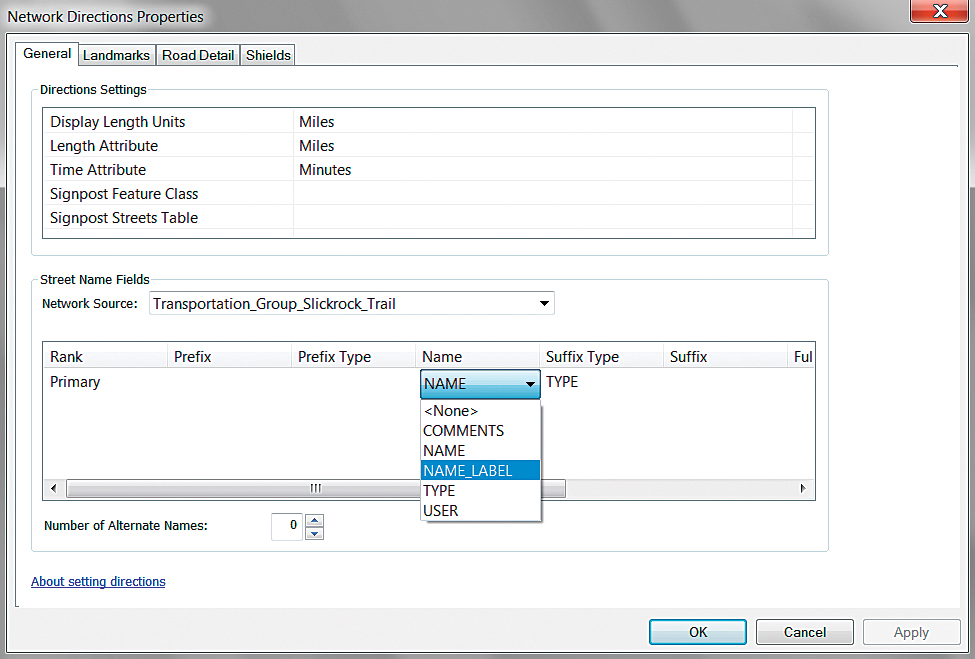
7. Now for the tricky part. Setting Directions will require reassigning the Name field to a predefined field in each dataset called NAME_LABEL and click the Direction button. For each network source (Slickrock Trail, Jeep Trails, Grand Co Roads), click the NAME header and select NAME_LABEL from the drop-down. Click OK, then Next, one more time.
8. Review the New Network Dataset Summary and click Finish. When asked to build the new network dataset, click Yes. Close ArcCatalog when processing has finished.
Rounding up Resources
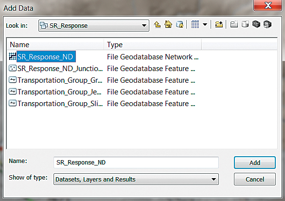
1. Restart ArcMap and open the Slickrock_Rescue map. Click Add Data, navigate to the Slickrock_Rescue\GBDFiles\ UTM83Z12\GC_Transportation\SR_Response feature dataset, and add SR_Response_ND. When prompted to add other participating feature clases, click No. Do not add other participating feature classes because the necessary ones are already in the map.
2. Right-click on an open area of the Standard toolbar and open the Network Analyst toolbar. This toolbar will be used to perform most of the rescue mapping tasks. Dock the Toolbar in the upper left, above the TOC.
3. Using the Network Analyst toolbar, open the Network Analyst window and park it to the right of your TOC. If you wish, you can use the toolbar’s Route function to test the network’s performance by dropping two or more points anywhere on the map, including the Bike Trail, and routing between them. Now formally test the network by using the Network Analyst Closest Facility (CF) function to locate emergency responders and route them to appropriate assembly points.
Running Closest Facility Backward
The training data includes the locations of 14 fictional Grand County SAR members who live throughout the Moab Valley. They are symbolized by rank inside green circles. The SAR operations base, symbolized with a black square, is 2.5 miles south of Moab at the Grand County Emergency Operations Center (EOC) on US Highway 191. The commander lives “just across the road.” To route SAR personnel from their homes to the EOC, we will reverse the typical Closest Facility workflow. This process will accumulate an effective response force and estimate the typical lead time required to assemble responders.
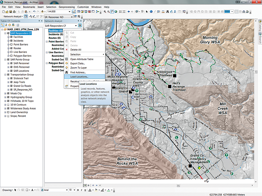
1. In the Network Analyst toolbar, click the drop-down and select the Closest Facility solver. The empty CF solver will load at the top of the TOC and appears in the Network Analyst window. Double-click Closest Facility in the TOC and open its Properties. Change the Layer Name to SAR Responders CF and close the Properties window.
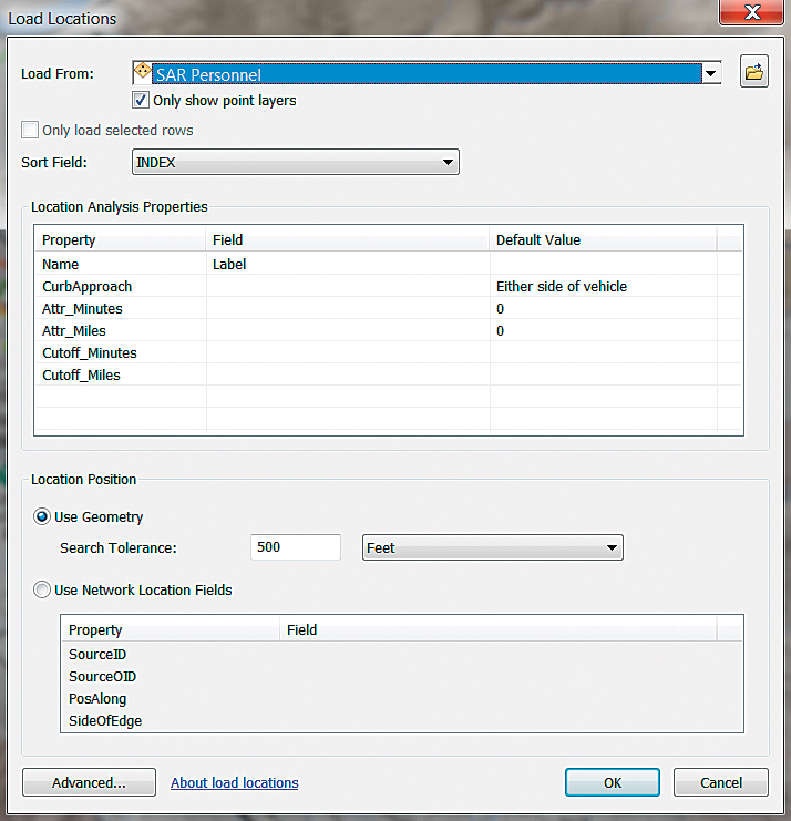
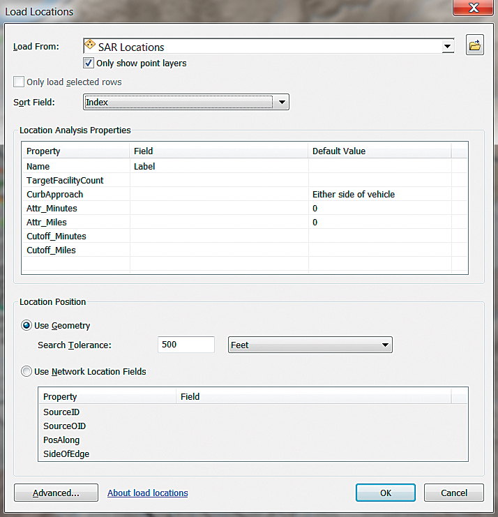
2. In the Network Analyst window, right-click Facilities. (Yes, Facilities is correct because this CF analysis is being run backwards.) Select Load Locations. In the Load Locations window, choose Load From to SAR Personnel. Set the Sort Field to Index, the Name to Label, and the Search Tolerance to 500 Feet. Click OK and watch the 14 personnel points load.
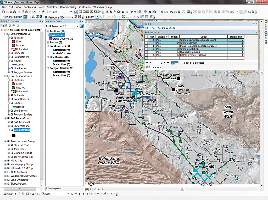
3. Right-click Incidents > Load Locations. In the dialog box, set Load From to SAR Locations and set Sort Field to Index and Name to Label. Click OK, and six incidents will load.
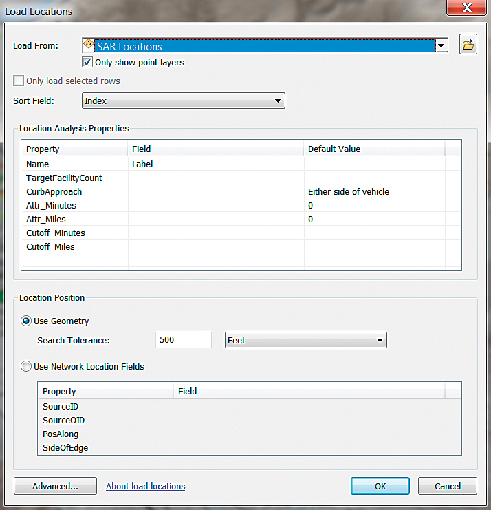
4. To retain only the Grand Co Emergency Management incident, open the Incidents set in the Network Analyst window, select all records except Grand Co Emergency Management, and delete them. Deleting unwanted records makes the IncidentID field much more functional.
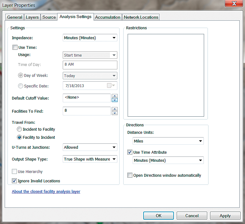
5. Double-click on SAR Responders CF to open its properties and select the Analysis Settings tab. Click the radio button next to Travel From to Facility to Incident and set Facilities To Find to 8. Keep the other defaults. (Hint: You may change the Output Shape Type from the default True Shape with Measure to True Shape; Straight Line, creating a traditional spider diagram; or to None, which is sometimes useful for very large CF routines.) Click the Accumulation tab and select both Miles and Minutes. Click OK to close Properties.
6. Now to route SAR responders. In the TOC, right-click SAR Responders CF and click Solve. The solver should quickly execute and create eight polyline routes from SAR residences to the Grand Co Emergency Management.
7. In the SAR Responders CF, right-click Routes, open its table, and position it at the top of the canvas and resize fields as necessary to make all of each record visible. (This is when a second monitor is helpful.) Be certain that the records are sorted by FacilityRank in ascending order.
8. Inspect the TotalMinutes field and notice that four responders can be routed to the EOC in under two minutes and six responders in less than three and all eight responders should arrive in less than four minutes. These are travel times to the facility only. Remember them and close the Routes table. Now use the Closest Facility routing procedure for EMS Personnel.
Routing EMTs to the Ambulance
The residences of 10 fictional Grand County EMTs, symbolized with blue circles, are located throughout Moab Valley. Most live within the city limits, so their travel time to the ambulance downtown garage should be minimal. The ambulance garage is labeled Grand County EMS.
1. To route EMS responders, create a second Closest Facility solver. In the Network Analyst toolbar, click the drop-down and select the Closest Facility solver. Double-click on the empty CF solver at the top of the TOC to open its properties and change its name to EMS Personnel CF.
2. In the Network Analyst window, right-click Facilities, select Load Locations, and choose EMS Personnel. Set the Sort Field to Index, the Name to Label, and the Search Tolerance to 500 Feet. Click OK.
3. Use the same procedure to load the Incident locations using SAR Locations. Delete all incident locations except Grand County EMS.
4. Open EMS Personnel CF, click the Analysis Settings tab, specify Facility to Incident, and set Facilities To Find to 6. Close Properties, right-click EMS Personnel CF, and choose Solve.
5. Open the Routes table and select two EMTs, who will make up the first team to reach the ambulance. Note that their travel times are less than two minutes. If additional EMTs are required for a multiple casualty incident, additional personnel will require slightly more travel time to reach a second or third ambulance.
Staging
Running the Network Analyst Closest Facility in reverse modeled travel times for SAR and EMS personnel traveling from their homes to base facilities. When modeling an actual response to a SAR incident, the arrival times of reponse personnel at the trailhead or other staging area must be coordinated so they will arrive at appropriate times. Knowing how long it takes SAR and EMS responders to drive to their base will allow determination of reasonable minimum total response times to each facility.
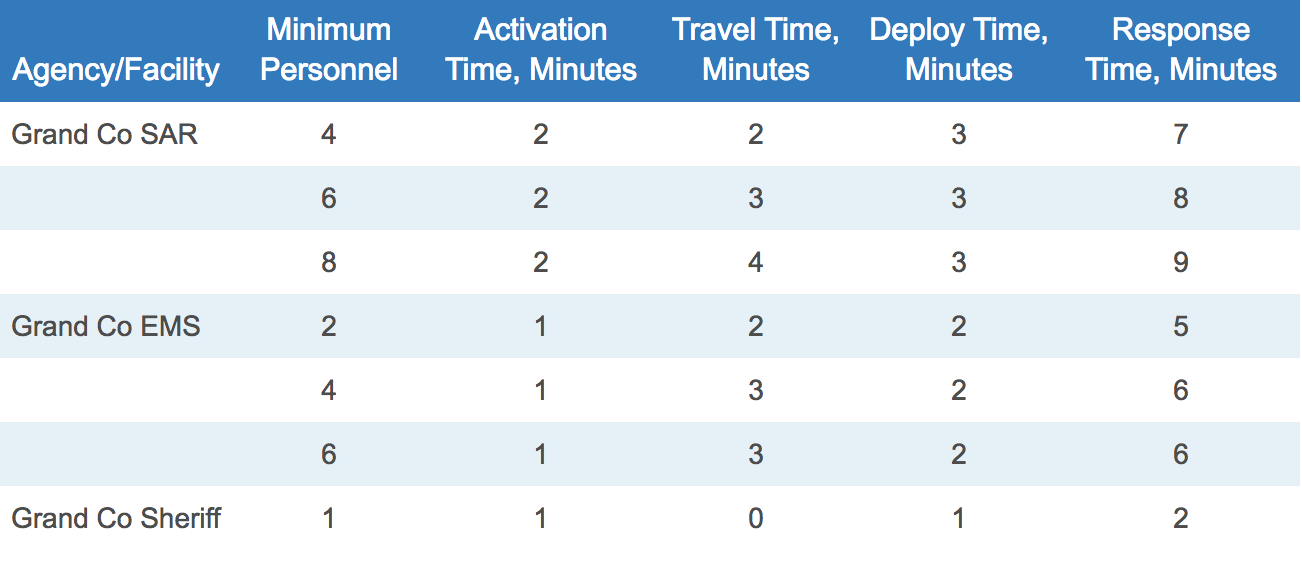
Table 1 lists response times for three county agencies, with options for several personnel counts. Total Response Time represents the time required for a responder to grab their gear and get out the door (Activation), drive to the facility (Travel), and prepare their vehicles for deployment (Deploy). A Grand County sheriff’s deputy, also added to the mix, quickly responds directly from the sheriff’s Office.
Lag times for minimal deployments can be entered into the attribute table for SAR Locations. Right-click SAR locations, select Edit Features > Start Editing, and open the attribute table. In the Delay_Min field, enter 7 for Emergency Management, 2 for the Sheriff, and 5 for EMS. When finished, choose Stop Editing from the Editing Toolbar. Save the map.
Summary and Acknowledgments
This tutorial teaches an intermediate-level user of the ArcGIS Network Analyst extension how to define and build a multimodal network dataset that models time and distance-based travel throughout the Slickrock area of Moab, Utah.
Special thanks to the Grand County, Utah, agencies that have supported the development of this response scenario and training set. Participating Grand County agencies include the Grand County Sheriff’s Office (especially Search and Rescue), Emergency Management, Emergency Medical Services, the Sand Flats Recreation Area team, and the Road Department. I could not have created this exercise without their excellent technical assistance and support.