What You Will Need
- Access to an ArcGIS Pro license
- Sample dataset downloaded from the ArcUser website
- Unzipping utility
- PDF reader
In September 2018, Graham Fire & Rescue (GF&R), the fire district for a small but rapidly growing community in Washington, was awarded a grant of more than $3.5 million from the Federal Emergency Management Administration (FEMA). GIS analysis and mapping done by the district was used to support the grant application.
GF&R is a fire protection district for the community of Graham located in Pierce County, Washington, approximately 40 miles southeast of Tacoma. (See the accompanying article “About Graham Fire & Rescue” for more information about GF&R and the SAFER program.)
In this tutorial, you will create several planning and presentation maps similar to the ones used for the GF&R grant application. Although some of the data used in the tutorial is synthetic, it represents conditions in and near Graham, Washington.
Getting Started
Download the sample dataset from
esri.com/arcuser and unzip it on a local machine, keeping the root path as short as possible.
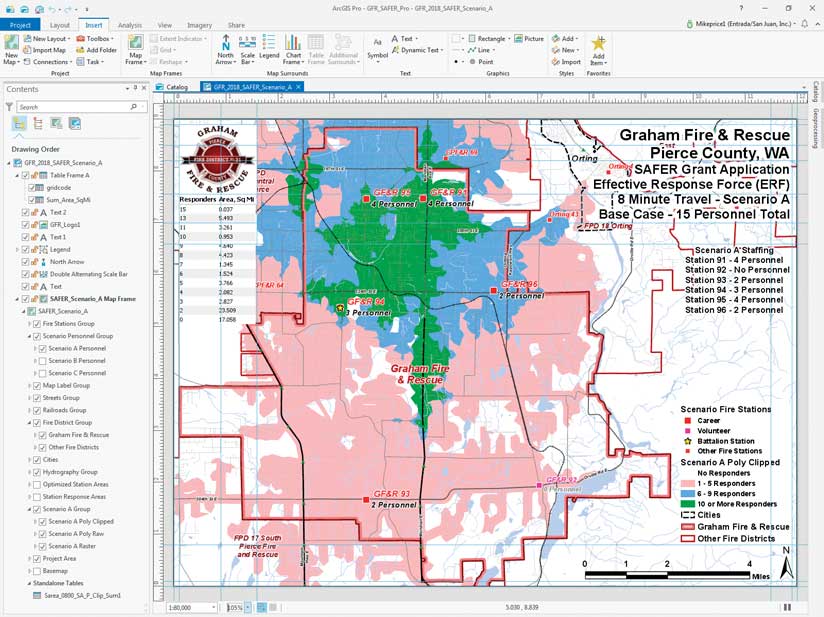
Start ArcGIS Pro and open the project, GFR_SAFER_Pro.aprx, and then open the GFR_2018_SAFER_Scenario_A layout. This map layout shows Scenario A, the current GF&R effective response force (ERF), which consists of 15 available responders who travel eight minutes from their assigned stations. Inspect the layout and study data layers, titles, and the current Responders table, sorted in descending order on the Responder field.
It shows the current travel coverage for Scenario A, including five career stations (i.e., stations staffed by nonvolunteers) with current staffing. Areas are colored to represent the number of responding personnel available in eight minutes. The area covered by 1 to 5 responders is shown in pink, and the area covered by 6 to 9 responders is symbolized in blue. The minimum desired number of GF&R personnel for a first alarm is 10 firefighters, and it is shown in green. The Responders Area Sq Mi table summarizes the area covered, listed by responder count.
GF&R encompasses 70 square miles. The total area covered by 10 or more firefighters is 9.74 square miles, or approximately 14 percent of the fire district’s area. Notice that the green areas are in the northwest portion of the district. This is where many Graham residents live and work.
Export a presentation PDF showing GF&R’s current staffing. With GFR_2018_SAFER_Scenario_A selected, click the Share tab and click Layout Export. Set Resolution to 200 dpi, check Embedded Fonts, select Best Image Quality, and click Export. Keep the layout name GFR_2018_SAFER_Scenario_A, and store the PDF in GFR_SAFER\Graphics. Open the exported PDF in Adobe Acrobat Reader or another PDF viewer.
On the Layout tab, click Activate in the Map section to open the map associated with the GFR_2018_SAFER_Scenario_A layout. The Map tab will be activated. Click Bookmarks and choose the GF&R SAFER 1:80,000 bookmark from the drop-down. Use this bookmark whenever you need to return to the full project extent.
Assessing Staffing Alternatives
This exercise adds up to four additional firefighters to selected career stations and tests the effects of increased coverage. In Scenario B, two personnel are added. In Scenario C, four personnel are added. Mapping and analyzing these scenarios will involve copying and modifying the Scenario A map and layout. Presentation graphics showing the effects of the proposed staffing increases will also be prepared.
Before considering future staffing scenarios, review current assigned station response areas and compare them to optimized travel times that were previously modeled using ArcGIS Network Analyst.
In the Contents pane, turn off Scenario A Group and turn on Station Response Areas and Optimized Station Areas layers located farther down the Contents pane. Solid colors shown by the Station Response Areas layer identify current assigned response zones for all six stations. Colored outlines shown by the Optimized Station Areas layer display optimized Network Analyst travel boundaries. Notice the close alignment of assigned zones and optimized travel.
To balance the workload against assigned areas, recent incidents could represent risk and be used to tabulate response load in each station’s assigned area.
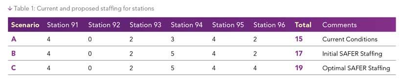
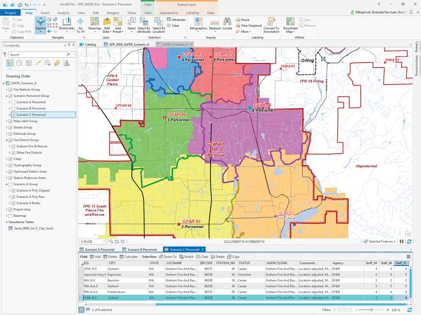
In the Contents pane, under the Scenario Personnel Group, turn on only Scenario A Personnel, and open its table. Scroll the table to the right and locate the Staff_SA field, which shows the 15 assigned personnel for the current deployment. Keep scrolling right and the Staff_SB field shows staffing for Scenario B, which adds two additional firefighters to Headquarters Station 94 for a total of 17 responders. The Staff_SC field shows staffing for Scenario C, which adds four additional firefighters to Station 96, giving a total of 19 responders. Table 1 summarizes current and proposed staffing for six stations.
Turn off Station Response Areas and Optimized Station Areas layers, and all layers in the Scenario Personnel Group. Save the project.
Modeling Proposed SAFER Staffing Scenarios
To model the two additional scenarios, create multiple copies of both the Scenario A map and layout. Fortunately, the legend for Scenario A was designed to display as many as 25 responders, so it can readily accommodate increased staffing without modification.
- If it is not already visible, turn on the Scenario A Poly Clipped layer (located in the Scenario A Group). It shows the eight-minute responder coverage clipped to the GF&R boundary.
- Click the View tab and open the Catalog pane (not the Catalog View), expand Maps, and right-click the SAFER Scenario A map. Choose Copy from the context menu. Right-click Maps and choose Paste to create a copy of the map. Repeat the process to make a second copy.
- Expand Layout and repeat the process to make two more copies of the GFR_2018_SAFER_Scenario_A layout.
- Rename the copies of the maps as SAFER_Scenario B and SAFER_Scenario C and the layouts as GFR_2018_SAFER_Scenario B and GFR_2018_SAFER_Scenario C. Be sure to rename maps and layouts in alpha order (from A to C). Save the project.
Defining and Refining Scenario B
This tutorial does not teach modeling travel using ArcGIS Network Analyst. The necessary raster and vector travel data has been included in the sample dataset in SAFER.gdb.
In the Catalog pane, under Layouts, right-click GFR_2018_SAFER_Scenario B, and choose Open.
- In the Contents pane, under GFR_2018_SAFER_Scenario B, right-click SAFER_Scenario_A Map Frame, and choose Properties.
- In Format Map Frame, click the first icon for Options, and under General, rename it SAFER_Scenario_B Map Frame.
- Under Map Frame, click the drop-down and set the data source to Map SAFER_Scenario_B. Save the project.
- Return to the Contents pane and double-click Text 1. In the Format Text pane, modify the text label to read 8 Minute Travel—Scenario B, Initial SAFER Staffing—17 Personnel Total.
- In the Scenario Personnel Group, turn on Scenario B Personnel to see the proposed staffing of all stations. Open Text 2 and update Station 94 staffing to 5 Personnel. Save the project.
- Creating and Updating Scenario B Polygons
- In the Contents pane, scroll down and turn off all layers in Scenario A Group, located below the Station Response Areas layer.
- Rename Scenario A Group, and the Poly Clipped, Poly Raw, and Raster layers from Scenario A to Scenario B by right-clicking on each, choosing Properties, and modifying the name. Turn on all layers.
Converting a Raster to a Polygon Layer
- Right-click Scenario B Raster, and open Properties. Click Source > Set Data Source. Click Folders under Project and choose GFR_SAFER > GDBFiles > WASP83SF > SAFER.gdb, and set the data source to Sarea_0800_SB, a raster. Click OK. Save the project.
- In the Catalog pane, expand Maps and open SAFER_Scenario_B. Click the Analysis tab ribbon, and click Tools.
- In the Geoprocessing pane, use the Search box to locate and open the Raster to Polygon tool in Conversion Tools.
- In the Raster to Polygon tool pane, set Input raster to Scenario B Raster, Field to Value, and set output as Project > Folders > GFR_SAFER > GDBFiles > WASP83SF > SAFER.gdb and name it Sarea_0800_SB_P_Raw. Check Simplify polygons, and click Run to build raw Scenario B 8-minute polygons. Sarea_0800_SB_P_Raw is added to Contents, symbolized as a single color. Turn this layer off.
- Make Scenario B Poly Raw visible, and right-click to open its Properties and select Source. Set the new Source to Sarea_0800_SB_P_Raw. The desired response force, shown in green, expands to include an additional area in the central portion of the fire district. Adding two responders to Station 96 helps a lot.
Clipping Polygon to District Boundaries
- Return to the Geoprocessing pane and use the Search box to locate the Clip tool in Analysis Tools > Extract).
- In the Clip pane, click the drop-down for Input Features and scroll down to choose Scenario B Poly Raw near the bottom of the list.
- Set Clip Features to Fire District Group\Graham Fire & Rescue.
- Set the Output Feature Class to Folders > GFR_SAFER > GDBFiles > WASP83SF > SAFER.gdb and name it Sarea_0800_SB_P_Clip, and click Run. It is added to Contents symbolized as a single color. Turn this layer off.
- When finished, turn on Scenario B Poly Clipped layer and change its source to Sarea_0800_SB_P_Clip, the clipped raster just created. Save the project.
Calculating and Summarizing Clipped Areas
Open the attribute table for the Scenario B Poly Clipped layer. Right-click the header for the gridcode field, and sort it in descending order. The gridcode field represents the number of available responders. The Shape_Area field gives the area of individual polygons. Notice that there are more than 1,000 polygons in this dataset.
Let’s add a new double precision field, calculate each polygon’s area in square miles, and summarize areas for all gridcode responder values.
- With Scenario B Poly Clipped highlighted in the Contents pane, click the Table tab and click Add.
- A new field is added at the bottom of this table. Name the field Area_SqMi; make its alias Area, Sq Mi; and set its Data Type to Double. Click in the Number Format, to bring up the Number Format pane and choose Numeric from the drop-down. Set Rounding to three decimal places, set alignment to Left, and check the box next to Pad with zeros. Click OK.
- Change the alias for the gridcode field to Responders.
- Uncheck Visible for ObjectID, Shape_Length, and Shape_Area. Check visible for gridcode and Area_SqMi, and uncheck Read Only.
- On the Fields tab on the ribbon, click Save to update the table. Close the Fields: ScenarioB tab.
- In the updated Scenario B Poly Clipped table, right-click the Area, Sq Mi field, and select Calculate Geometry.
- Set Input features as Scenario B Poly Clipped; set Target Field to Area, Sq Mi; set Property to Area; and set Area Unit to Square Miles (United States). Set the Coordinate System to the Current Map. Click Run to calculate areas.
- Once the Area, Sq Mi field is populated with values, right-click the Responders header, and choose Summarize. In the Geoprocessing pane for Summary Statistics, set the Input Table to Scenario B Poly Clipped, and set output path to Folders > GFR_SAFER > GDBFiles > WASP83SF > SAFER.gdb and name the output table Sarea_0800_SB_P_Clip_Sum1. Set the Statistics Field to Area, Sq Mi; set the Statistic Type to Sum; and verify that the Case field is Responders. Click Run to create the summary table.
Scroll the Contents pane down, expand Standalone Tables, and open the Sarea_0800_SB_P_Clip_Sum1. Sort gridcode in descending order. Compare the Responders count to the sum of Area_SqMi.
Let’s update this table’s appearance. Click the Table tab on the ribbon and click Fields. Set Responders as the alias for gridcode. Set Area, Sq Mi as the alias for Sum_Area_SqMi, and click Numeric in the Number Format column to bring up the Number Format pane. Set Rounding to 3 Decimal places, Alignment to Right, and check the box next to Pad with zeros. Turn off visibility for OBJECTID and FREQUENCY. Click Save in the ribbon to update the summary table. Close the Geoprocessing and Catalog panes.
Close Fields: Sarea_0800_FER_Scenario_B). In Sarea_800_SB_P_Clip_Sum1, select all records that have 10 or more responders. Right-click Area, Sq Mi, and select Statistics. Above the chart, click the Selection Filter tab. In the Chart Properties pane, select Sum. It has a value of 14.39 square miles. This is the response area covered by 10 or more responders in Scenario B compared to Scenario A coverage of 9.74 square miles. Close the Chart Properties pane, tables, and the chart, and save the project.
Placing Tables in a Layout
- Let’s add the Scenario B table to the Scenario B layout. Activate the layout by clicking the SFR_2018_SAFER_Scenario B tab. Turn off Table Frame A in the Contents pane. In Contents, select Standalone Table Sarea_0800_SB_P_Clip_Sum1.
- Click the Insert tab on the ribbon, and click Table Frame. Use your cursor to draw a rectangle to position the table. Outline the rectangle immediately below the GF&R logo and approximately the width of the logo, and extend it to the 5-inch ruler mark. When you release the mouse button, the table will appear.
- In the Contents pane, rename the Table Frame to Table Frame B. Next, reformat the table by right-clicking it, and opening its Properties.
- On the Format Table Frame pane:
- Click the icon on the far right to reset its placement width to 1.5 and its height to 2.5. Set X to 0.1 and Y to 7.55.
- Click the third icon from the left to set the display. In that pane, scroll to the bottom of the pane and set both Background 1 and Background 2 to white.
- Click the second icon from the left to set alignment. Expand Sorting, click the plus sign and add gridcode, and uncheck ascending. Leave all other settings unchanged, and close the Format Table Frame pane. Inspect the updated table and save the project.
Exporting a Scenario B Map
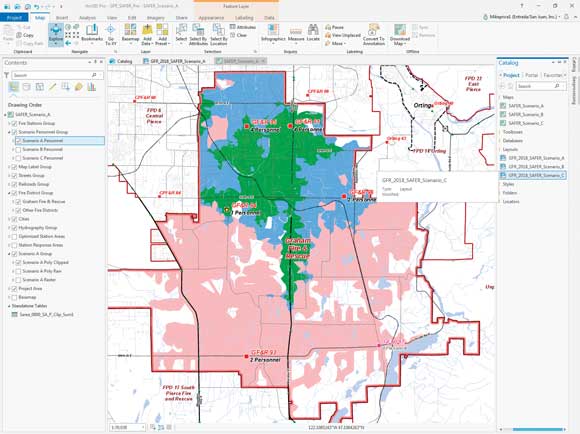
Now export the completed Scenario B map to a presentation PDF file. Inspect the Scenario B layout and verify that all titles are correct. Turn on Scenario B Personnel and Scenario B Poly Clipped. Open the Catalog pane and expand Layouts. Right-click GRF_SAFER_Scenario_B, and select Export to File. Navigate to GFR_SAFER, and save the file using the Layout’s name.
Open the file in a PDF reader and confirm that items have been updated in Scenario B. If you find any items that need to be updated, close the PDF file, move to the project’s root directory (to release a possible PDF lock), and return to your project. Make the necessary changes, save your project, and export again.
On Your Own
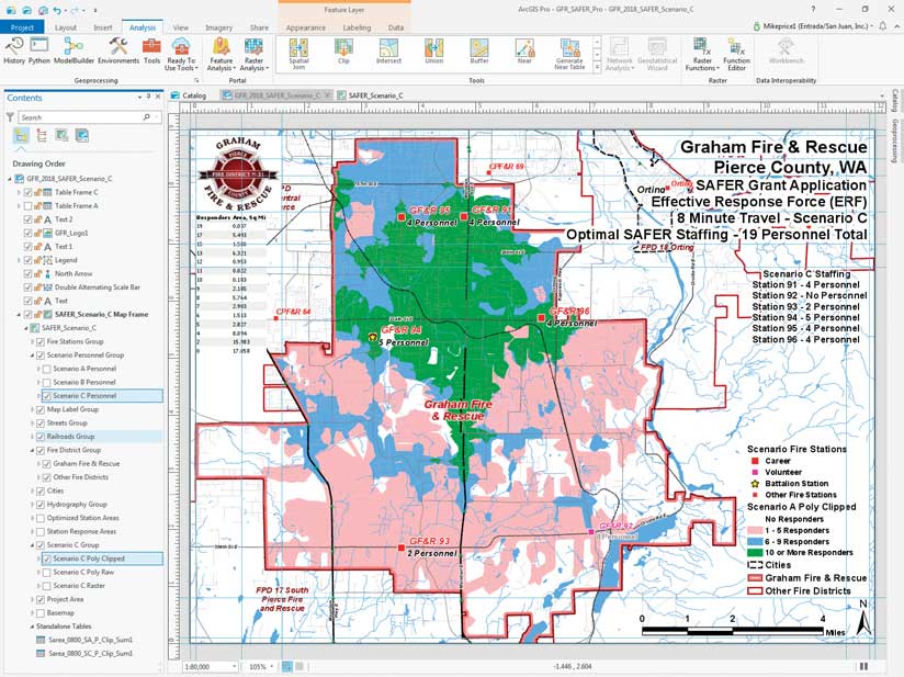
Now it’s your turn to create a Scenario C map using the same workflow described in this tutorial. You will update one map and one layout for Scenario C. Title this map: 8 Minute Travel—Scenario C, Optimal SAFER Staffing—19 Personnel Total. Update Text 2 to reflect that Station 96 staffing has four added personnel for a total of 19 responders.
Remember to closely follow file naming rules to keep the scenarios separate. When finished, verify that the statistical Area, Sq Mi sum for 10 or more responders for Scenario C is approximately 14.59. Notice the moderate extension of area covered by 6 to 9 responders (shown in blue) and the large increase in area covered by 1 to 5 responders (shown in pink). Save the project one last time, and export the Scenario C map to complete the presentation set.
Summary
Congratulations. In this tutorial, you created three very persuasive presentation maps that show how GF&R might staff up to meet the needs of the rapidly growing community of Graham, Washington. Remember, although this exercise is strictly hypothetical, it does show how the real the needs of GF&R could be addressed.
Acknowledgments
I commend GF&R for receiving the SAFER grant and the fine service that it provides to this growing jurisdiction. Thanks to assistant chief Oscar Espinosa and the GF&R staff for help with this exercise. Thanks also to the GIS data managers in Pierce County, Washington, for providing datasets that helped represent real-world conditions.
I commend Chief Espinosa for providing planning, data integration, and technological support for the district. I respect his commitment to an ArcGIS Pro deployment “right out of the box,” without having prior experience with ArcGIS Desktop. This has truly been a rewarding learning experience. I have certainly developed new workflows and teaching tricks, and I’ve learned a lot in the process.