Calculating the difference between bare earth and first return lidar rasters provides information such as forest canopy height and character, building heights and orientation, aboveground utility alignment, a count of cars on the road, and even estimates of large livestock in a field.
This tutorial teaches how to use bare earth and first return lidar rasters to compare natural and cultural features in ArcGIS Pro. It uses data from previous ArcUser tutorials that was collected in 2017 during a public safety event sponsored jointly by agencies in the United States and Canada called the fifth Canada-United States Enhanced Resiliency Experiment (CAUSE V) exercise. For more information on this exercise, see “Testing Cross-Border Disaster Response Coordination” in the fall 2017 issue of ArcUser.
A tutorial in the fall 2017 issue of ArcUser, “Modeling Volcanic Mudflow Travel Time with ArcGIS Pro and ArcGIS Network Analyst,” used CAUSE V data to model volcanic mud and debris flows (lahars), riverine flooding, landslides, and other natural phenomena caused by the hypothetical crater collapse of nearby Mount Baker.
The rasters enabled CAUSE V geoscientists and emergency managers to accurately predict lahar behavior and identify values at risk along its travel path. They were collected by WSI (Watershed Sciences, Inc.). The company was contracted by the Nooksack Indian Tribe and the Puget Sound LIDAR Consortium (PSLC) to collect lidar data along the Nooksack River Basin, which was flown in 2013. This exercise makes further use of that lidar data.
Getting Started
Download the sample dataset from the ArcUser website and unzip it on a local machine. The archive includes a new prebuilt ArcGIS Pro project, two lidar surfaces, and four georeferenced drone images. In this exercise, make sure to follow the naming conventions specified.
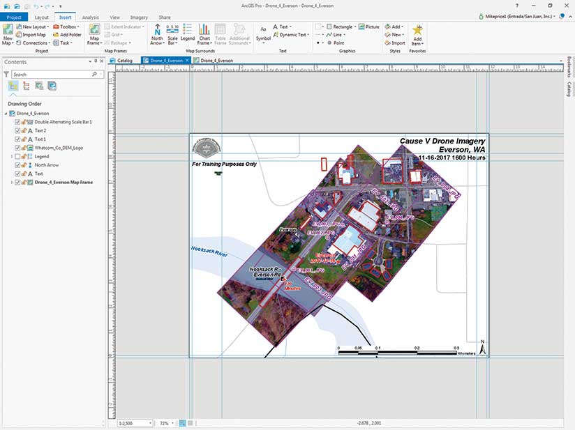
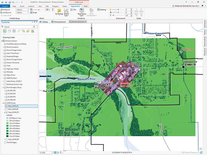
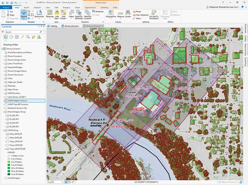
Start ArcGIS Pro and open Drone_4_Everson.arpx, located in CAUSE_V_Drone_4\Drone_4_Everson. The project displays the four georeferenced drone images. Inspect the layout and notice how the georeferenced images closely match the river corridor and building footprints. How would you confirm the location and position of natural and cultural features on these images? This exercise uses bare earth and first return lidar rasters to do that.
Switch from the Drone_4_Everson layout to the Drone_4_Everson map, and inspect the feature layers in the Contents pane. The coordinate system is universal transverse Mercator (UTM) North American Datum 1983 (NAD83) Zone 10 N. All horizontal and vertical units are in meters. Turn individual images on and off and zoom in to check the georeferencing accuracy. Turn on the Esri World Imagery basemap and compare it to the drone imagery.
On the ribbon, click Project and select Options. In the Options window, open the Map and Scene window and make sure the scene type is set to Local.
Global scenes display 2D and 3D data using the World Geodetic System 1984 (WGS 84) Web Mercator (Auxiliary Sphere) coordinate system. Local scenes display data that has a spatial reference in a local projected coordinate system with terrain and layers projected on a planar surface. Local scenes support display and analysis of data at a large scale and within a fixed extent.
ArcGIS Pro will retain this local scene selection, so be sure to switch back to a global scene if you model small-scale data subsequently, especially if data is referenced in a geographic coordinate system (GCS) rather than supported in a local scene. Click the back arrow located in the upper-left corner and save the project.
Adding Lidar Rasters
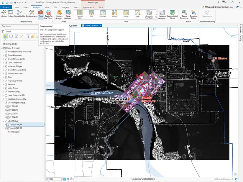
In the ArcGIS Pro map, click the Add Data button, navigate to \CAUSE_V_Drone\GDB_Files\UTM83Z10, and open Topo_LiDAR.gdb. Hold down the Shift key and select Topo_LiDAR_BE (the bare earth raster) and Topo_LiDAR_FR (the first return raster). Click OK to add them to your map.
After the lidar rasters load, select both, right-click either layer, and choose Group. Rename the new group LiDAR Group and place Topo_LiDAR_FR above Topo_LiDAR_BE.
First return points are typically positioned above the bare earth. Check the elevation range for each raster. Each raster has 1-meter resolution and contains considerable detail. Move Lidar Group below Drone Imagery Group and save the project.
Modeling Lidar Hillshade
Hillshades show the high level of detail in both rasters and visually demonstrate the difference between first returns and bare earth. Create hillshade rasters for both lidar surfaces. In the ArcGIS Pro ribbon, click the Analysis tab, and select Tools to display the Geoprocessing pane. In the Contents pane, highlight Topo_LiDAR_FR and type hillshade in the Geoprocessing pane’s Search window to locate the Hillshade tools for Spatial Analyst and/or 3D Analyst. Although there are several ways to display a hillshade in ArcGIS Pro, you need either the Spatial Analyst extension or 3D Analyst extension to perform other tasks in this workflow.
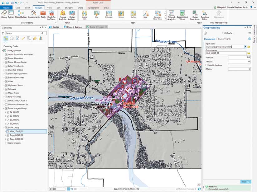
In the Geoprocessing Hillshade pane, set the Input Raster to Topo_LiDAR_FR and specify the Output raster Hlsh_LiDAR_FR. Make sure you save it in Topo_LiDAR.gdb. Leave other parameters unchanged and click Run.
After the first return hillshade is added to the Contents pane, move it just above Topo_ LiDAR_FR and inspect it briefly. Return to the Geoprocessing Hillshade pane and create a hillshade for Topo_LiDAR_BE and name it Hlsh_LiDAR_BE. (Hint: Simply change FR to BE in both raster windows.) In the Lidar Group, place Hlsh_LiDAR_BE immediately below Hlsh_LiDAR_FR and save the project.
Enhancing Lidar Symbology
Since the bare earth and first return rasters contain reasonably similar elevation ranges, the same classified symbology can be applied to both using a layer file. In the Contents pane, make only Topo_ LiDAR_FR visible, and right-click this raster and select Symbology to open its pane. In the Symbology pane, click the menu bar in the upper-right corner (which is three horizontal bars).
Click Import, navigate to \CAUSE_V_Drone\GDB_Files\UTM83Z10, and select Lidar Topo Symbology.lyr. Click OK to apply, and repeat the process for Topo_LiDAR_BE.
Turn off Topo_Lidar_BE. Turn on Hlsh_LiDAR_FR and select it. On the Raster Layer tab, click the Appearance tab and in the Effects area, set the transparency to 50 percent. Turn on Hlsh_LiDAR_FR and Topo_LiDAR_FR. Inspect the visual enhancement provided by the partially transparent hillshade. Also set the transparency of Hlsh_LiDAR_BE to 50 percent in the same manner. Turn on Hlsh_LiDAR_BE and Topo_LiDAR_BE. Save the project.
Creating and Enhancing Contours with Barriers
Now, let’s create bare earth contours. The Contour with Barriers tool provides a highly functional way to create index and intermediate contours, even if you do not assign barriers. Reopen the Geoprocessing pane, type contour in the Search window, and select Contour with Barriers from either the Spatial or 3D toolset. Select Topo_LiDAR_BE (not Hlsh_LiDAR_BE) as the Input Raster, skip Input Barrier Features, and name the Output Contour Features Con_Topo_LiDAR_BE. Set the Base Contour to 0, the Contour Interval to 1, and the Index Contour Interval to 5. Click Run to create the contours.
In this project, I have provided a Contour Line template, stored as a layer file. Once the contours build and display, click the Add Data button, navigate to \CAUSE_V_Drone\GDB_Files\UTM83Z10, and add LiDAR Topo BE Contours.lyr. If you have followed the naming and storing conventions exactly, the contour lines should reload with appropriate symbology and labels. If the layer has a red exclamation point next to it, indicating a broken data source, right-click it, choose Properties > Source and click Set Data Source. Navigate to the location where you saved Con_Topo_LiDAR_BE and set the data source to that location. If it still does not load properly, start troubleshooting by verifying that files have been named correctly.
Remove Con_Topo_LiDAR_BE from the Contents pane, relocate LiDAR Topo BE Contours below NDH Flowlines, and save the project again.
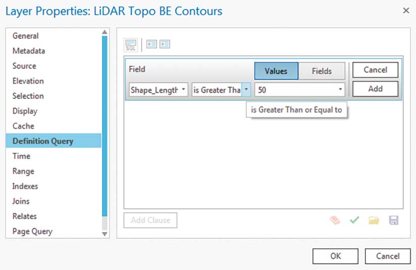
Notice that there are many small closed contours, even in the relatively simple bare earth set. To remove the smallest contours, create a definition query to display contours that have a length of 50 meters or more.
In the Contents pane, right-click LiDAR Topo BE Contours, select Properties, and open Definition Query. Click Add Clause and create a query where Shape_Length is Greater than or Equal to 50. Click OK, and the smallest contours should disappear. Notice how contour lines often match the bare earth raster’s unique values thematic symbology. This is certainly reassuring. Save the project again.
As a challenge exercise, you could contour and symbolize the first return raster. Expect that it will be very noisy.
Calculating the Difference between First Returns and Bare Earth
One of my favorite lidar tasks is calculating the difference between the first return and bare earth rasters because it yields information that is useful in the real world.
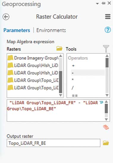
Return to Geoprocessing tools and type raster calculator in the Search window. Select Raster Calculator (the raster calculator from either the Spatial Analyst or 3D Analyst extension toolsets will work).
In the Raster Calculator window, create an expression that subtracts Topo_LiDAR_BE from Topo_LiDAR_FR. The expression order is critical. Make sure that you use the minus sign operator. Store the Output raster in Topo_LiDAR.gdb and name it Topo_LiDAR_FR_BE. Click Run to model the difference in the two rasters.
After Topo_LiDAR_FR_BE loads in the Contents pane, change its symbology by applying the layer file LiDAR Feature Height FR-BE.lyr. Move it to the bottom of the LiDAR Group.
In the next step, create one more contour set that will emphasize the differences between first returns and the bare earth. Before creating detailed contours, turn off LiDAR Topo BE Contours and use Bookmarks to zoom in to Everson 1:2,500.
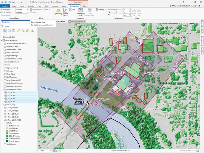
Once zoomed in, turn on the Drone Imagery Group and select all four images. On the Raster Layer tab, click the Appearance tab, and in the Effects area, set the transparency for all drone images to 75 percent.
Return to the Geoprocessing Contour with Barriers tool and create another contour set by setting Input Raster to Topo_LiDAR_FR_BE, Output Contour Features to Con_Topo_LiDAR_FR_BE, Base Contour to 0, Contour Interval to 2, and Index Contour Interval to 10. Click Run to create contours.
To symbolize and label contours, load another layer file template. Navigate to \CAUSE_V_Drone\GDB_Files\UTM83Z10 and load LiDAR Height Contours.lyr. Place the new layer above LiDAR Topo BE Contours and remove Con_Topo_LiDAR_FR_BE. Notice how height contours define riparian woodlands, building footprints, the Highway 544 bridge, cars on roadways, logs in the river, and maybe even a cow or two. Save once more.
Exporting and Reviewing a Lidar Map
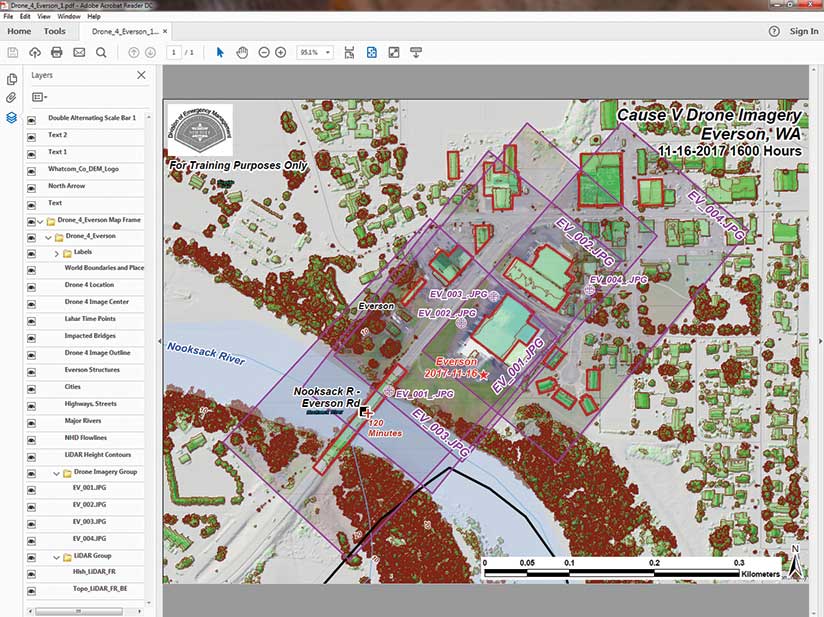
To export the map, click the Everson_4_Layout tab and inspect your layout. Open the Catalog pane and expand Layouts. Right-click Drone_4_Everson and select Export to File. Save the export file as a PDF with a resolution of 300 dpi. Place it in \CAUSE_V_Drone\Graphics and name it Drone_4_Everson_1.pdf. Because the map has a lot of detail, it may take some time to generate the PDF.
Open a file manager such as Windows Explorer and browse to \CAUSE_V_Drone\Graphics. Open Drone_4_Everson_1.pdf. Click the Layers icon and use the visibility selection (eye symbol) to turn individual layers off and on. Investigate how the ArcGIS Pro PDF export function manages labels, images, analytical rasters, and transparency. Compare the lidar height contours to Everson structures and the georeferenced images. They should match pretty closely thanks to the 1-meter resolution of the rasters. Continue to explore the PDF export, and consider how you might use the workflow presented in this article.
If you were wondering why the cars in the lidar rasters aren’t in the drone imagery, remember that the lidar was acquired in 2013, while the drone imagery was flown in 2017. Any cars or cows shown in the 2013 lidar rasters were long gone when the drone imagery was captured.
Summary
This is certainly one of my favorite ArcUser exercises. I took traditional ArcMap workflow tasks and updated them directly in ArcGIS Pro. I am especially thankful for the robust online help included with ArcGIS Pro. I encourage you to use it whenever you need extra assistance.
Acknowledgments
Thanks again go to the CAUSE V team members for all their support and encouragement. Thanks also to WSI (Watershed Sciences, Inc.), the Nooksack Nation, and the Puget Sound LIDAR Consortium for acquiring and hosting the great lidar dataset that supports this exercise.