This tutorial demonstrates how ArcGIS Pro can generate multiple layouts from a single project and incorporate more sophisticated layer transparency. It uses individual response type layouts created in the spring 2017 issue of ArcUser and adds custom contour polyline datasets for each density raster. The updated layouts are exported as PDFs.
Fire and emergency medical service (EMS) providers carefully analyze emergency responses in time and space. To optimize resources and provide the best level of service, equipment and personnel are positioned to provide the best service possible. To understand the frequency and density of emergency and nonemergency responses, public safety GIS staff categorize and map incidents by incident type. Mapping incidents to understand historic demand for services is the best way to provide a reasonable estimate of future service requirements.
Exercise Overview
In the Spring issue of ArcUser, an existing ArcMap document containing 6,300 emergency response calls was imported into ArcGIS Pro for additional analysis. Incidents were coded based on the National Fire Incident Reporting System (NFIRS). Multiple layouts were created from the project and exported as PDF documents for printing and presentation.
Kent Fire Department (KFD) generously allowed the use of a slightly synthetic subset of its emergency calls records for current and previous exercises. The department protects a rapidly growing group of communities approximately 20 miles southeast of Seattle. The area is characterized by a mix of single family and multifamily residences, retail/commercial, industrial, warehousing, and other occupancies.
KFD is noted for developing and deploying many best practices in the fire service and has shared its knowledge with the GIS community. KFD is the cornerstone of a large fire and EMS protection group named the Puget Sound Regional Fire Authority (PSRFA). The PSRFA uses GIS extensively to map and understand public needs; plan for future growth; and manage its staff, apparatus, and other resources.
This exercise uses the ArcGIS Spatial Analyst Kernel Density geoprocessing tool to model all five risk sets created in the last tutorial from 2016 responses in the core KFD coverage area. This exercise will show how to generate custom contour polyline datasets for each density raster. The individual response type layouts created in the last exercise will be updated with this data and exported as PDFs.
Getting Started
Begin by downloading the sample dataset from the ArcUserwebsite. Use this dataset rather than the final version of the dataset from the previous exercise because several new layer files have been added and are needed for this exercise. Unzip the dataset and save it locally in a new folder so the previous exercise data is not overwritten.
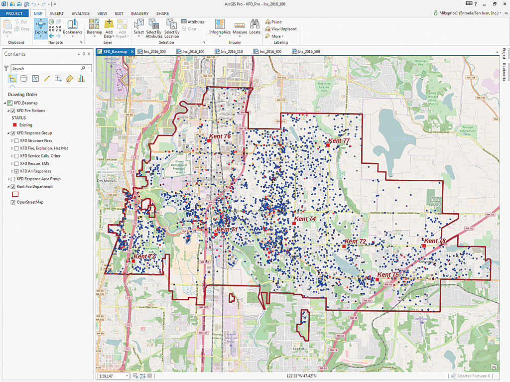
In Windows Explorer, browse to KFD\KFD_Pro\ and double-click KFD_Pro.aprx to open it. Inspect the project and note the layouts for five NFIRS incident groups. If necessary, repair any disconnected data links. Turn off the OpenStreetMap basemap and turn on KFD Fire Stations, KFD Response Group, and KFD All Responses.
Setting Up Geoprocessing in ArcGIS Pro
Click the Analysis tab in the ribbon and click Tools. The Geoprocessing pane should load on the right side of the workspace. Maximize its length if necessary. Click Toolboxes and scroll down to locate and expand the Spatial Analyst toolbox. These tools require an ArcGIS Spatial Analyst license. Notice that these tools are similar to ones made available when using the Spatial Analyst toolset in ArcMap.
Expand the Density group. Hover over the Kernel Density tool to read its description but do not open it. Collapse the Density tools and expand the Surface tools (also in the Spatial Analyst toolbox). The Surface set includes three contouring tools including Contour with Barriers. Hover the cursor over Contour with Barriers to read its description. This exercise will not use barriers but will use other advanced features of this contouring tool. Leave the Spatial Analyst toolbox open.
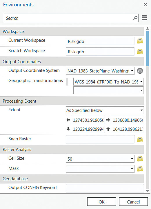
Click Environments in the ribbon on the Analysis tab. Before performing spatial analyses, several processing parameters and limits must be set. The parameters in this pane are similar to the Environment settings in ArcMap. Workspace, Output Coordinates, Processing Extent, and Raster Analysis must be specified before modeling the data.
In Environments, set the Current and Scratch Workspaces by navigating to \GDBFiles\WASP83NF and setting both parameters to Risk.gdb. Click the Output Coordinate System drop-down and select Kent Fire Department. The coordinate system is now Washington State Plane NAD83 North US Feet. This will be changed. To make sure that any data in World Geodetic System (WGS 1984) will be properly transformed, click the Transformations dropdown and select WGS_1984_(ITRF00)_To_Nad_1983, which is located near the bottom of a very long list.
Next, use the drop-down to set the Processing Extent to Kent Fire Department. For Cell Size, type 50. This will define a cell containing a call location equal in size to the width of a typical four-lane street. Click OK to save changes and close Environments. Save the project to preserve these settings.
Modeling and Contouring Incident Density
In the 2016 emergency response dataset, each point represents a unique response to an emergency or a service call. Responses are also captured at the apparatus level, so one incident may have two or more records that reflect each unit assigned to an incident. Mapping incident density typically models filtered data so that each point represents one emergency response or service call known as a master event. The dataset of master calls includes false calls and events cancelled in route and are categorized in a Service Calls, Other subset.
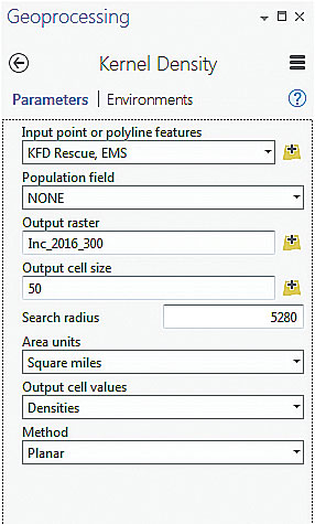
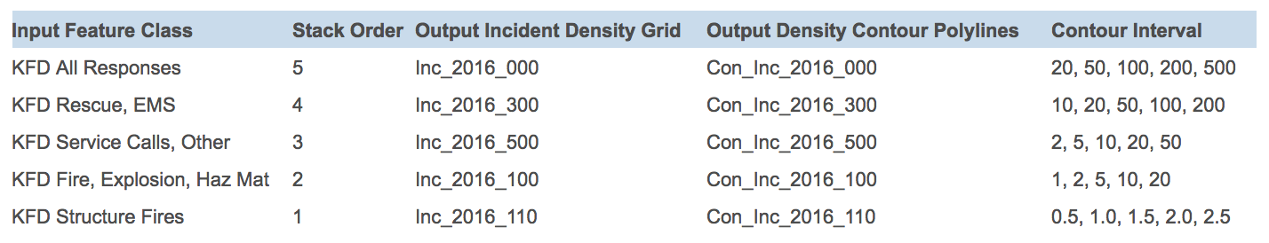
Return to the Geoprocessing pane, collapse Surface tools, and expand Density tools. Click Kernel Density. In the Kernel Density wizard, select KFD All Responses as Input features, leave the Population field as NONE, and name the Output raster Inc_2016_000. Make sure it is being saved to the Risk geodatabase as previously specified. The Output cell size should be 50 (so it will match the size set in Environments), set the Search radius to 5280 and Area units to square miles. Accept defaults for other parameters, click Run, and watch as the Kernel Density tool creates the Inc_2016_000 grid and loads it into the Contents pane. Save the project and return to the Geoprocessing pane.
Create four more density rasters using the Kernel Density tool and information in Table 1 to determine what to name the output incident density grids for each input feature class. After running the Density Kernel tool for each item, organize the output rasters as shown in the Stack Order column of Table 1 with 5 located at the bottom of the table of contents. Don’t modify the symbology.
To check your work, turn on each raster and input set individually, and study the relationships between input points showing individual incidents and the density rasters generated from them. Open the Catalog pane (the Project pane in ArcGIS Pro 1.4) and expand Geoprocessing History to see five Kernel Density items. The most recent raster should be at the top of the list. Hover over each raster to verify its parameters. Save the project.
Creating Cool Contours
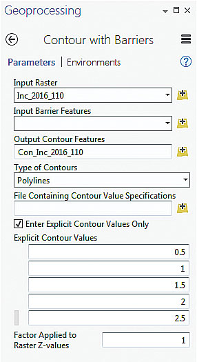
Now to model contours for all five rasters. Use the back arrow in the Geoprocessing pane to return to all the toolboxes and expand the Surface toolset. Select Contour with Barriers. This tool is the most advanced contouring tool in the toolbox. Although barriers won’t be used, this tool is used to manually define discrete contour intervals.
Select Inc_2016_110 (which is the density raster for structure fires) as the Input Raster, name its output Con_Inc_2016_110, and make sure it will be saved to the Risk geodatabase. Check the box next to Enter Explicit Contour Values Only. Refer to the values listed under Contour Interval in Table 1 for the interval values. Type 0.5 in the first textbox below Enter Explicit Contour Values Only and press Enter to set that value and open a new textbox. Continue inputting the rest of the values under Contour Interval for KFD Structure Fires in Table 1. Make sure to click inside the new textbox each time to give it the focus, enter the interval value, and press Enter each time to create five intervals. Click Run.
After Con_Inc 2016_110 loads in the Contents pane, open its attribute table. Contour values range from 0.5 to 2.5. Type code 3 represents discrete user-defined intervals. If you need to add or remove an interval, you could return to the current Geoprocessing pane, make changes, and run the process again. Close the attribute table, turn off Con_Inc 2016_110, and save the project.
Use the Contour with Barriers tool to create contours for Inc_2016_100 (Fire, Explosion, Haz Mat) and make sure to rename the output as Con_Inc_2016_100. Change the explicit contour values to 1, 2, 5, 10, and 20 as specified in Table 1. These values accommodate nonlinear, somewhat logarithmically distributed data. Continue modeling the three remaining rasters, making sure to use the contour intervals from Table 1.
At the bottom of the Geoprocessing pane, click the Project tab to display the Catalog pane. In the folder list in the Catalog pane, expand the Geoprocessing History folder. Notice that the list includes five new Contour with Barriers events. Save the project.
Enhancing and Printing Incident Density Maps
The five density rasters and density contour sets could be manually symbolized. However, if Group Layer files have been created in ArcMap to preserve symbology, they could be used by loading them into the project and repairing any broken links.
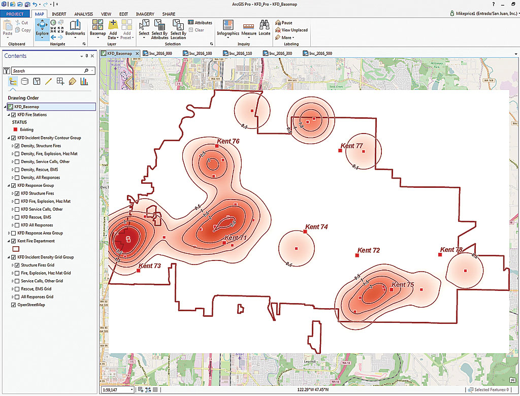
Click the Map tab in the ribbon and choose Add Data > Data. Navigate to \GDBFiles\WASP83NF and locate KFD Incident Density Contour Group.lyr and KFD Incident Density Grid Group.lyr. Add these layer files using the map Contents pane. Move KFD Incident Density Contour Group to a spot just below the Con_Inc_ files. Move KFD Incident Density Grid Group to a spot just under the Inc_2016_ files. Expand both groups and notice that each group contains five layers and all have broken links.
Repair each layer in the KFD Incident Density Contour Group by right-clicking on it in the Contents pane; clicking Properties; and, in the dialog, clicking Source. Connect each layer in the KFD Incident Density Contour Group to the appropriate Con_Inc_2016 feature class just created and stored in \GBDFiles\WASP83NF\Risk.gdb. Once all the KFD Incident Density Contour Group data links have been repaired, make sure all Con_Inc_ files are turned off and turn on each KFD Incident Density Contour Group to make sure they are correctly linked. If they are, remove all Con_Inc files from the project.
Use the same methodology to repair the source data link for the layers in KFD Incident Density Grid Group by connecting them to the appropriate Inc_2016_ file geodatabase raster in the Risk.gdb, referring to Table 1. Turn each relinked layer off and on individually to make sure they are correctly linked and then remove the Inc_2016_ files from the project.
Study the color, symbology, and label for each line, which were imported from the layer file. Check all five layer file rasters and contour sets to ensure they have been correctly linked. Remove the temporary geoprocessing data (i.e., the density and contour files just linked to the layer files). Turn on the OpenStreetMap base and save the map. Notice that the raster transparency originally defined in the layer file imported from ArcMap is not respected.
Applying Raster Transparency (and an ArcGIS Pro Shortcut)
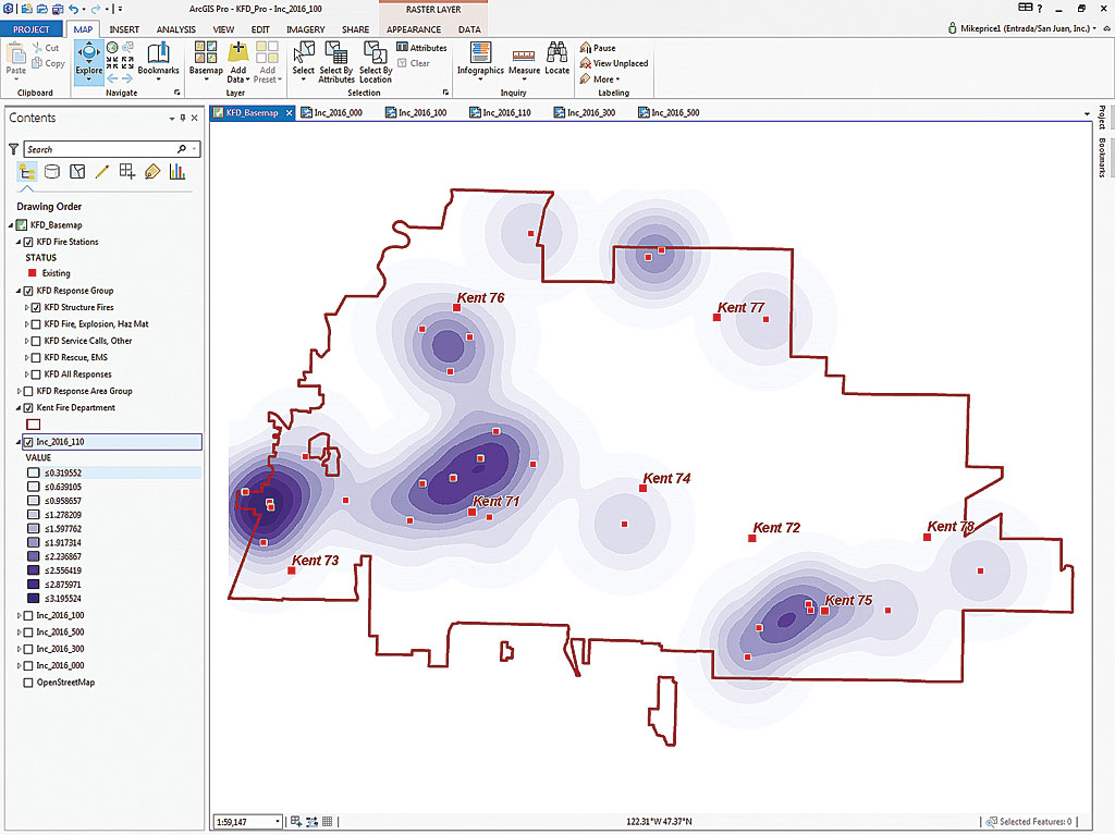
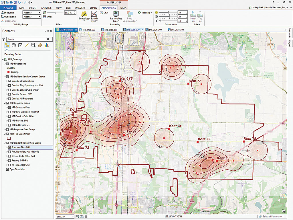
In ArcGIS Pro, raster and vector transparency is assigned through tools in the Appearance ribbon. To change a raster’s appearance, select Structure Fires Grid from the KFD Incident Density Grid Group and click on the Appearance tab in the ribbon. In the Effects section, change transparency from 0 percent to 50 percent. Press the Enter key to set the percentage, and the transparency will update. The partially transparent raster enhances the appearance of the point density raster. The labeled contour lines suggest density even when the raster and points are not visible. Contours certainly enhance presentation maps for a mixed audience.
Instead of adjusting transparency for the remaining four density grids manually, use this shortcut. In the Contents pane, select all five density grids by holding Shift (to select a range of adjacent layers) or Ctrl (to select each layer individually). Return to the Effects tool on the Appearance ribbon to set transparency for all selected rasters to 50 and press Enter. Make sure all density grids are updated. Save the project again.
Exporting Multiple Layouts
In the previous tutorial, incident maps were exported from five separate layouts. Each layout was designed and titled for a specific incident type. This exercise uses the same layouts to export maps that include incident density grids and density contours. To do this, each layout will be individually activated and updated to make specific KFD Response Group items visible, including the density raster and contour layer, before being exported or printed.
To create a map showing density and contours for structure fires, make sure the Density, Structure Fires, KFD Structure Fires, and Structure Fires Grid layers are all visible. Right-click the Inc_2016_110 tab on top of the map canvas. Verify that the layout’s subtitle is Structure Fires.
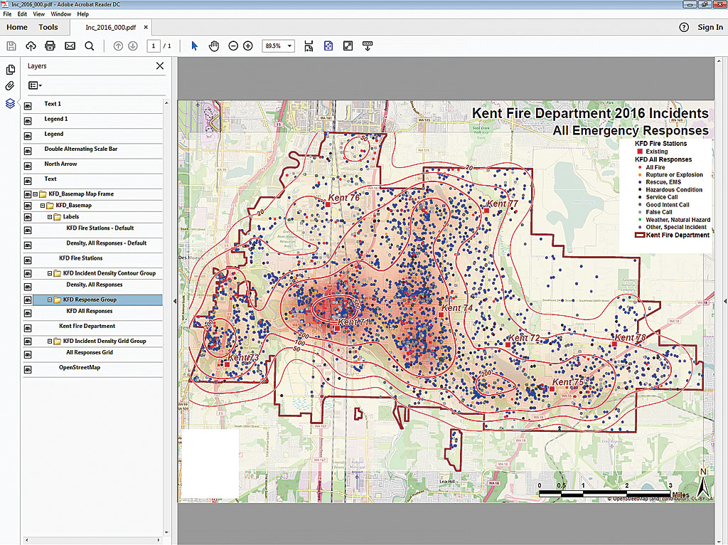
Open the Catalog pane by clicking the Project tab on the right size. Expand Layouts and right-click KFD_Inc_2016_110. Choose Export to File. In the Export Layout wizard, navigate to \KFD and create a new folder called Graphics. Set resolution to 200 dpi, verify that Embed Fonts is checked, and click Export. Use Windows Explorer to locate the file, and use Acrobat Reader or another program that can open PDF files to view the exported map.
To understand the power and function of ArcGIS Pro’s updated PDF export, open one of the exported PDF maps. Notice that all visible layers are included in the PDF as individual elements that can be turned on and off independently rather than merged into a single PDF object titled Image when exported as a PDF in ArcMap.
For each of the four remaining layouts, update which layers are visible based on Table 1. Select the tab for the appropriate layout, right-click it, and choose Activate. Export each, accepting the name of each layout as the exported file’s name. When finished exporting layouts, save the project. View the updated exported files by navigating to KFD\Graphics.
Summary
This ArcGIS Pro exercise builds on the previous one with additional modeling, contouring, and mapping of incident density. Imagine ways that these maps could be used to identify stations with the greatest number of EMS, fire, and other calls. These maps provide excellent performance measurement and operations planning tools.
Acknowledgments
Thanks once again to the Kent Fire Department for the use of its great data. This sample dataset represent only one-third of Kent’s total responses for 2016 and should not be used to predict an actual response profile. Thanks also to Esri technical staff for their advice and support as I continue to investigate ArcGIS Pro.