What You Will Need
- An ArcGIS Pro 2.0 or 2.1 license
- ArcGIS Network Analyst license
- Sample dataset from the ArcUser website. [ZIP]
- Access to the Internet
On November 15 and 16, 2017, public safety agencies in the United States and Canada and supporting government and industry entities plan to conduct a training and proof-of-concept exercise along the westernmost border between the United States and Canada called the Canada-US Enhanced Resiliency Experiment (CAUSE) V. This is the fifth in a series of CAUSE exercises held since 2011.

This exercise will involve a hypothetical crater collapse on Mount Baker, a 10,781-foot (or 3,286-meter) dormant composite volcano, located approximately 30 miles (49 kilometers) east of Bellingham, Washington. Now ready for deployment, it will simulate the effects of several major structural collapse events near the mountain’s summit. The seismic activity that would accompany these events would result in volcanic mud and debris flows (lahars), riverine flooding, landslides, and other natural phenomena. Data from these events will be synthesized and sequenced to test response and recovery capabilities of the US and Canadian emergency agencies.
A significant result of the crater collapse would be several lahars, first in the western Nooksack River drainage and later in the Baker/Skagit River system of Mount Baker’s eastern side. A key part will include modeling the extent and travel times of these lahars in several drainage systems.
This tutorial introduces a special use of ArcGIS Network Analyst, an ArcGIS Pro extension, to route and measure a lahar originating above the Middle Fork of the Nooksack River. The travel model uses pre-built stream flowlines developed from the the National Hydrography Dataset (NHD). The empirical timing used in the exercise was developed from the study of a similar lahar that resulted from the May 1980 eruption of Mount St. Helens, also in Washington.
For more information about CAUSE V, see the accompanying article, Testing Cross-Border Disaster Response Coordination. For background information on Mount Baker, see the accompanying article Mount Baker (Briefly).
Modeling Lahar Flow with NHD Flowlines
This tutorial uses data from NHD, which is managed by the US Geological Survey (USGS) as part of The National Map. NHD is a high-resolution compilation of drainage networks and related features, including rivers, streams, lakes, ponds, glaciers, and dams. Flowline data provided by NHD includes seamless stream centerlines and nonflowing water centerlines. Flowline connectivity and directionality support hydrologic network modeling.
This tutorial uses modified NHD Stream, River, and Artificial Path vectors to model lahar travel in the Nooksack River drainage. The flowlines are edited in one area to allow the network to cross a minor drainage divide and enter the Sumas River drainage.
For more information about NHD or to obtain NHD data, visit the Hydrography page of The National Map at nhd.usgs.gov/index.html.
Getting Started
Download the sample dataset archive, Cause_V_Lahar.zip, from the ArcUser website to a local machine and extract the data. This archive contains several file geodatabases, a prepared stream centerline dataset, and an MXD document that will be imported into ArcGIS Pro.
Start ArcGIS Pro, make sure you have an ArcGIS Network Analyst license available and active, and create a new Blank project. When prompted to Create a New Project, name it Lahar_Model and store it in Cause_V_Lahar\GDBFiles\UTM83Z10. Make sure you store the new project in this folder.
Once the new project has opened, click the Insert tab, then click Import Map. Navigate to Cause_V_Lahar, select Lahar_Model_01.mxd, and click OK.
Once it has opened, inspect the imported map. It uses the same layout as the original map, and its current extent shows the Nooksack River flowing west from Mount Baker into Puget Sound. Also, notice that this map shows Johnson Creek and the Sumas River flowing northeast into British Columbia. Inspect the Cities, Towns, and Census Designated Places (CDPs) and CAUSE V Lahar Zones layers and turn on the NHD Flowlines layer. Look at the Collapse Points layer, and note the two collapse points located on Mount Baker and at the Lahar 01 Origin.
Open the Catalog pane, right-click Maps > Open to open Lahar_Model_01. All modeling in this tutorial will be done in map view.
On the Map ribbon, click the Basemap dropdown, and select Terrain with Labels. Although the Canadian terrain will flash momentarily and then disappear, the labels for the area remain visible.
Using NHD Flowlines to Define Lahar Travel
In the Contents pane on the left side of the interface, highlight NHD Flowlines Selected, right-click, and open its attribute table. Select individual records and study their attributes. Zoom in to check NHD flowlines in and near the communities of Everson and Nooksack. There is a very low drainage divide between the Nooksack River and Johnson Creek. The CAUSE V model will deflect part of the lahar flow out of the Nooksack drainage into the Johnson Creek/Sumas River drainage, and the flow will continue across the border between the United States and Canada and flow toward the Fraser River.
Next, close the attribute table and turn off NHD Flowlines Selected. Turn on NHD Flowlines All. In the Contents pane, expand the legend for NHD Flowlines All and open its attribute table. These polylines are raw NHD Flowlines, clipped along the Nooksack corridor. This dataset was filtered prior to the CAUSE V event to create the network dataset that will be used in this model.
Close the attribute table and turn off the NHD Flowlines All layer. Turn on the NHD Flowlines Lahar 01 layer and open its attribute table. Notice that this prepared dataset includes the same polyline data as NHD Flowlines Selected. The difference is that its attribute table supports time and distance network modeling. Sort the KPH (kilometers per hour) field in descending order.
Selecting High Velocity Flowlines
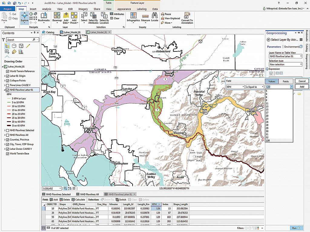
On the ribbon, click the Table tab then Selection by Attributes.
In the Select Layer by Attributes Geoprocessing pane, make sure Layer Name or Table View is set to NHD Flowline Lahar 01 and Selection type is set to New selection. Click the Add Clause button to bring up the expression creator. Create an expression choosing KPH for Field, then is Equal to, and select 120 as Value.
Click Run to select all records in which KPH is Equal to 120.
This selection includes the highest velocity flowlines located high on Mount Baker that begin at Lahar 01 Origin. In imperial units, 120 KPH is approximately 75 miles per hour (MPH) or nearly 110 feet per second.
Click the Map tab and use the Lahar 01 Origin 1:50,000 bookmark to zoom in and identify any flowline segment immediately below Lahar 01 Origin. Verify that all units are metric and that the velocity is 120 KPH. Notice the very short travel times.
Use the bookmark for Everson Nooksack 1:100,000 to zoom in and observe the constructed flowline vectors connecting the Nooksack River with Johnson Creek and Sumas River. These segments allow the lahar to travel over the Everson divide and continue north toward the Fraser River. Close the attribute table, save the project, and let’s begin modeling.
Empirical Lahar Travel Estimates
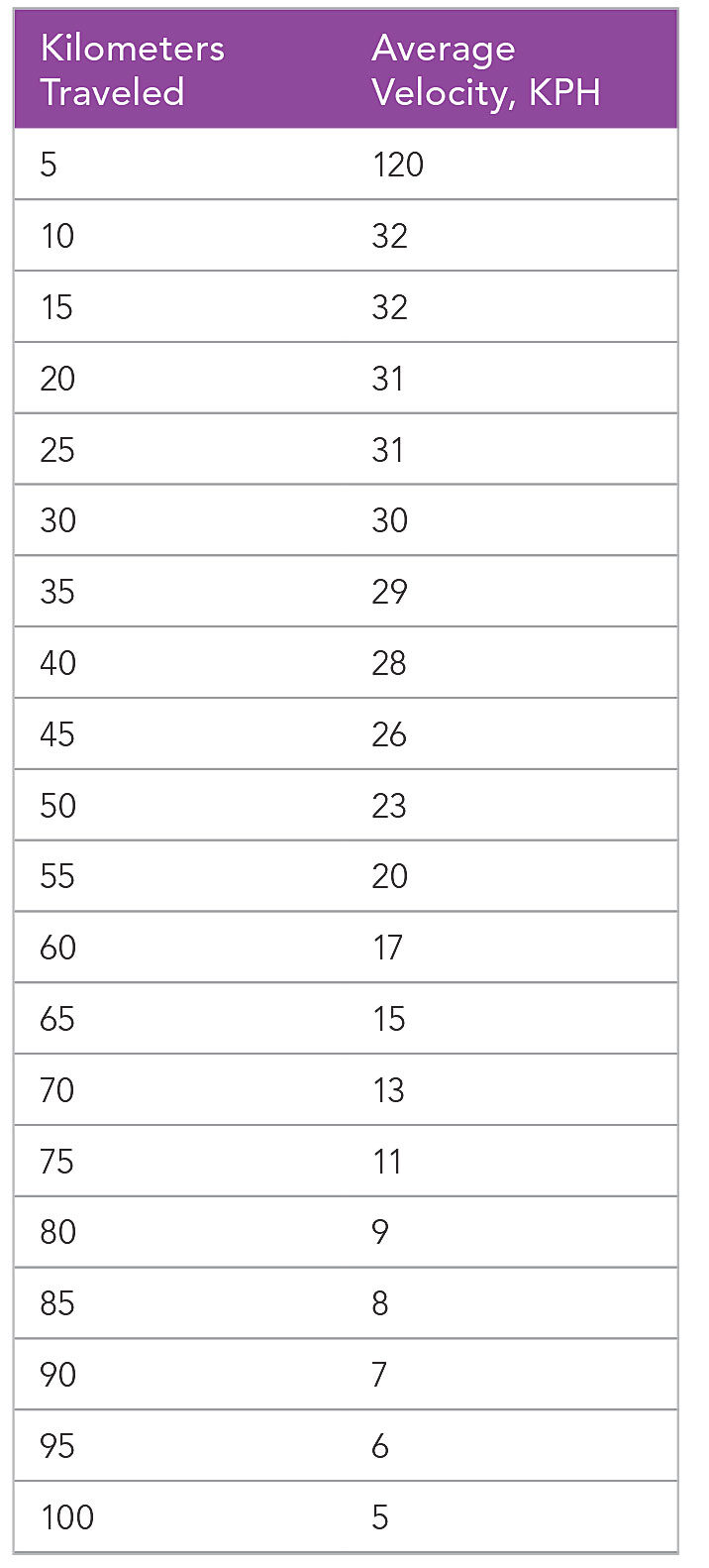
The model velocities that will be used to determine lahar timing are derived from studies of lahars on the North and South Forks of the Toutle River that were created by eruption of Mount Saint Helens on May 18, 1980. Dr. T. C. Pierson, a research hydrologist at the US Geological Survey’s Cascades Volcano Observatory, studied the Toutle River debris flows and developed distance-based velocities for a typical Cascade volcano lahar. His findings were published in a 1998 paper called An empirical method for estimating travel times for wet volcanic mass flows. Pierson’s findings are summarized in Table 1, which lists estimated velocities based on distances below the origin. These values were used to set velocities for selected stream segments in this tutorial.
Loading a Prepared Lahar Network Dataset
To streamline this tutorial, a metric network dataset using selected NHD flowlines was prepared and included in the sample dataset. It was edited to include the Everson crossing. Stream vectors extend from Lahar 01 Origin at Puget Sound in the west to the Fraser River in Canada. ArcGIS Network Analyst was used to determine the flow distances to assign the velocities shown in Table 1. Modeling another debris flow would require constructing a separate network dataset.
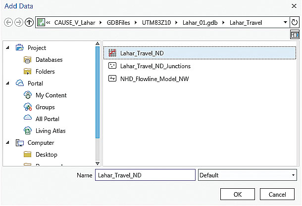
To load the prepared network dataset, on the Map ribbon, click the Add Data button and navigate to CAUSE_V_Lahar\GDBFiles\UTM83Z10\Lahar_01.gdb\Lahar_Travel.gdb.
Click Lahar_Travel.gdb and click Lahar_Travel_ND to add it.
After the network dataset loads, move this layer to just below the NHD Flowlines All layer in the Contents pane. Save the project.
Creating a Service Area Analysis Layer
Click Analysis on the ribbon and click Tools.
In the Geoprocessing pane, click Toolboxes, expand Network Analyst Tools, expand Analysis tools, and locate Make Service Area Analysis Layer.
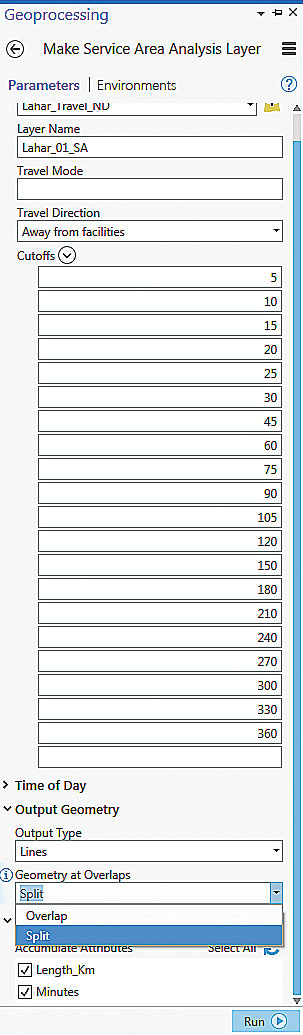
In the Make Service Area Analysis Layer pane, specify Lahar_Travel_ND as the Network Data Source. Name the Layer Lahar_01_SA, skip Travel Mode, and set Travel Direction to Away from facilities.
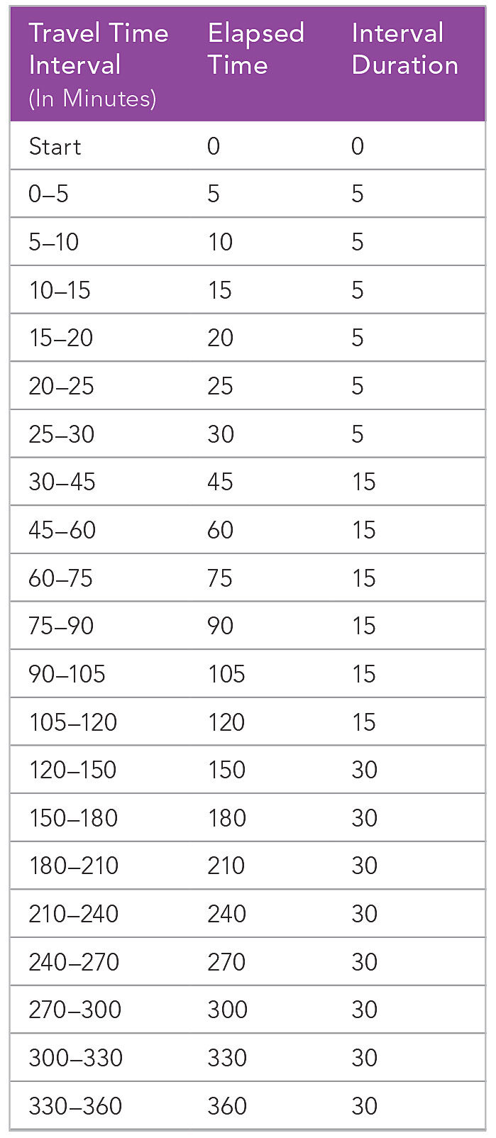
Still in the pane, under Cutoffs, accept the first three completed (5, 10, 15), type 20 in the first empty cell, and press Enter or Tab to open another cell. Continue typing values in subsequent cells under Cutoffs using the values in the Elapsed Time column of Table 2. Carefully enter these values, as they will be used in a definition query expression later in this tutorial.
Skip Time of Day and expand Output Geometry. Set Output Type to Lines and set Geometry at Overlaps to Split. Polygons do not work well here, so flowlines must be split using the cutoff values just entered.
Expand Accumulate Attributes, and check both Length_Km and Minutes.
Click Run. The Service Area Analysis Layer is created and loaded into the Contents pane. Save the project when finished.
Adding a Lahar Facilities Origin and Creating a Lahar Line Set
In the Contents pane, select the Lahar_01_SA to invoke the Network Analyst Service Area tab.
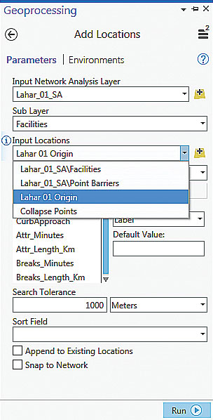
Click the Network Analyst Service Area tab on the ribbon and click Import Facilities.
In the Geoprocessing Add Locations pane, set Input Network Analysis Layer to Lahar_01_SA, set Input Locations to Lahar 01 Origin. Set Search Tolerance to 1000 Meters, leave Append to Existing Locations and Snap to Network unchecked, and leave other fields unchanged.
Click Run to add the Lahar 01 Origin point. A single point for Facilities loads over Lahar 01 Origin. Save the project again.
After the Facility point loads, locate and click Run on the Service Area ribbon and watch the network analysis execute.
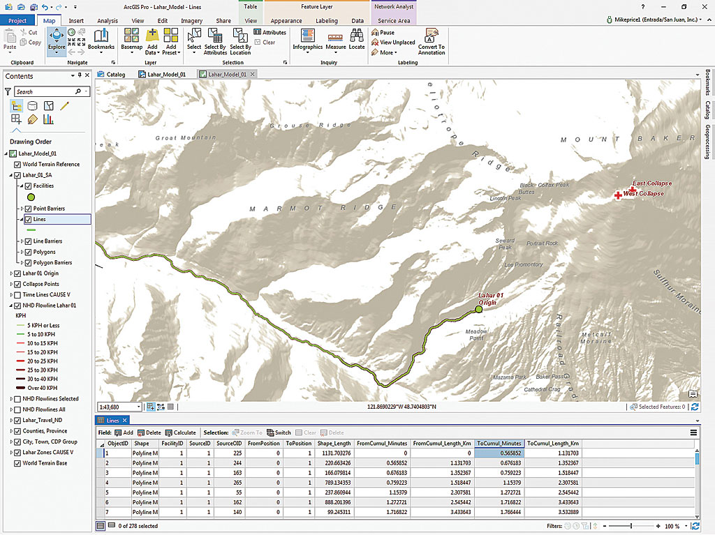
When it is finished, return to the Lahar_01_SA group in the Contents pane. Right-click Lines and open its attribute table, which should have 278 records. Inspect the Lines attribute table and explore the ToCumul_Minutes field. This field contains the downstream time for lahar travel on each NHD segment. Sort the field in ascending order and scroll through the values. You should see the time breaks as values of 5, 10, 15. If you do not see them all, rerun the solver, specifying Split for all Table 2 intervals.
Once the Lines layer values are validated, export Lines to a permanent polyline feature class. In the Lahar_01_SA group, right-click Lines, choose Data > Export Features. In the Copy Features Geoprocessing pane, set Input Features to Lines and save the polyline feature class in CAUSE_V_Lahar\GDBFiles\UTM83Z10\Lahar_01.gdb\Lahar_Travel.gdb as Lahar_01_SA_Lines.
Save the project again.

Calculating Endpoint Coordinates and Time Point Set
Now to assign endpoint coordinates to all exported Line vectors. Open the Geoprocessing pane and type geometry in the Find Tools box. This should return the Add Geometry Attributes at or near the top of the search list. Alternatively, locate the Add Geometry Attributes tool in the Features toolset, which is in the Data Management Toolbox.
In the Geoprocessing Add Geometry Attributes pane, specify Lahar_01_SA_Lines as Input Features and select Line start, midpoint, and end coordinates for Geometry Properties. Specify Meters as Length Unit and Square Meters as Area Unit.
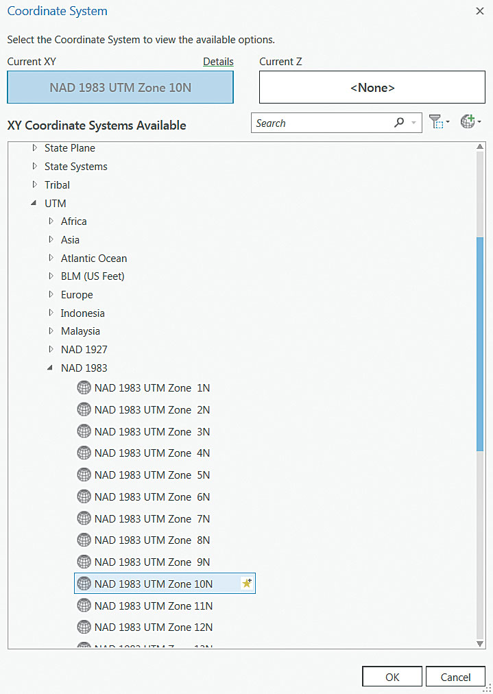
It is very important to set the Coordinate System to North American Datum 1983, Universal Transverse Mercator Zone 10N (NAD_1983_UTM_Zone_10N). Click the globe icon and in the Coordinate System pane, choose Projected > UTM > NAD 1983 > UTM Zone 10N.
When all fields and the coordinate system have been set, click Run.
When the processing is finished, scroll across the updated table and locate the END_X and END_Y fields. These fields contain UTM coordinates for vector downstream endpoints. By creating an x,y point set of selected endpoints, the desired time points can be posted on the map, but first, all vectors must be filtered to obtain the values listed in Table 2.
Click the Map tab on the ribbon and click Select By Attributes. Specify Lahar_01_SA_Lines as the Layer Name, set Selection type to New selection, and open the Expression window, which could be used to create the expression by clicking 5 for the first value, and clicking Add and continuing the process to create a similar expression for the rest of the 21 elapsed time intervals listed in Table 2.
Instead of doing all that work, load the prepared expression included in the sample dataset, which will perform this task. On the bottom line of the Select Layer by Attribute pane below the Expression text box, locate the folder icon and click it. Navigate to CAUSE_V_Lahar\Utility and load Interval_Times_Definition_Query.exp. Once the expression is loaded, inspect it, and click Run.
This query selects the 34 records that represent the desired time intervals. Return to the Geoprocessing search field and type copy rows to locate the Copy Row tools.
In the Copy Rows Geoprocessing pane, set Input Rows to Lahar_01_SA\Lines and Output Table to Lahar_01_SA_Lines_XY and save it in CAUSE_V_Lahar\GDBFiles\UTM83Z10\Lahar_01.gdb\Lahar_Travel.gdb. Zoom to the map display using the Nooksack R 1:250,000 bookmark.
Click Add Data and navigate to the Lahar_01_SA_Lines_XY table and add it to the map.
Make Event Layer
Right-click on the Lahar_01_SA_Lines_XY table in the Contents pane and choose Display XY from the context menu. In the Geoprocessing Make XY Event Layer pane, set the X Field to END_X and the Y Field to END_Y. Accept the default name of Lahar_01_SA_Lines_XY_Layer. Use the Counties, Province feature class to define the spatial reference. Click Run.
After the Event Layer loads in the Contents pane, check the locations of all points and save the project. To create a permanent layer, right-click the Lahar_01_SA_Lines_XY_Layer and select Data > Export Features. Save the new feature class in Lahar_01.gdb and name it Lahar_01_Time_Points. Be very careful to use this name: Lahar_01_Time_Points.
Do not load the new feature class in the map and use a layer file that will symbolize the data. Return to the Map ribbon, click Add Data, navigate to CAUSE_V_Lahar\GDBFiles\UTM83Z10\, and load Lahar 01 Time Points.lyr. The points will appear along the Nooksack and Sumas Rivers as black cross symbols with the modeled travel time at each point. Save once more.
Update CAUSE V Lahar Model Layout
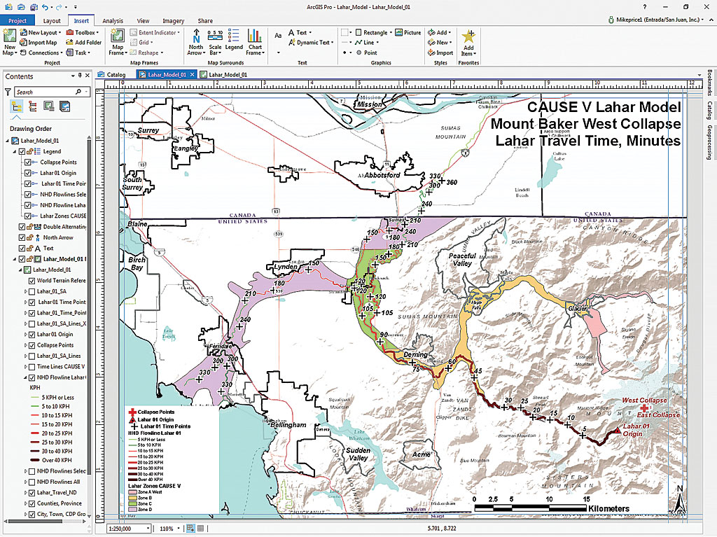
Finally, go to the Catalog pane, expand Layouts, and open Lahar_Model_01 to view the layout. Review the progress of the lahar over time as it descends the Middle Fork of the Nooksack River to the confluence with the North Fork at approximately 60 minutes. The flow continues on to the Everson/Nooksack area where it separates into two lobes at approximately 120 minutes. Follow each lobe as it continues on down the Nooksack toward Puget Sound or north into Canada along Johnson Creek and the Sumas River. Notice that as velocity decreases and deposition occurs along debris flow margins, it may take more than 300 minutes, or five hours, for lahar debris to reach Puget Sound and nearly six hours for debris to reach the Trans Canada Highway 1, east of Abbotsford, British Columbia.
Summary
The data presented and modeled in this exercise is completely hypothetical and is not intended to represent an actual event. Lahar travel times are approximately modeled using empirical observations and analyses of a recent actual explosion in the central Cascades.
Acknowledgments
The author thanks the agencies and staff that design and support CAUSE V, including Cascades Volcano Observatory; Whatcom County, Washington; Washington Emergency Management; and all other supporting agencies and organizations. Special thanks to Dr. T. C. Pierson and Cynthia Gardner at the Cascades Volcano Observatory.