“Editing with Feature Templates,” in the summer 2015 issue of ArcUser, introduced editing with feature templates and showed how editing templates are created, updated, and applied.
This article will expand your feature template editing skills and teach how to digitize structural geology features from scanned maps. This tutorial will cover symbolizing and labeling geologic points representing the orientation of bedded strata and geologic polylines used for representing simple and complex fault movement.
The previous exercise involved creating simple feature templates and modifying the line direction for existing small-scale faults. Working this exercise will involve digitizing detailed geologic data and creating new points and polylines. The mapped faults in the previous exercise were mapped at 1:100,000 scale, but in this exercise, features will be digitized at a scale of 1:24,000 or larger using a small part of a scanned graphic of the Antler Peak quadrangle.
Getting Started
To get started, download the Battle_Mountain09, Antler Peak training data [ZIP] and unzip it on a local drive.
Open ArcCatalog and navigate to \GDBFiles\UTM83Z11\Antler_Peak.gdb. Expand the geodatabase and preview the table for the faults and GeoPoints layers. Note that these are currently empty but will be populated during this exercise. Close ArcCatalog.
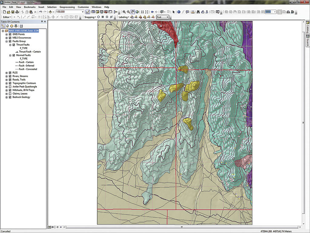
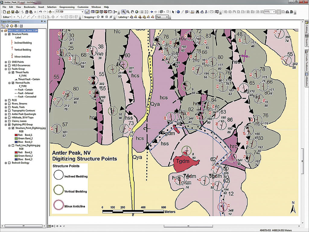
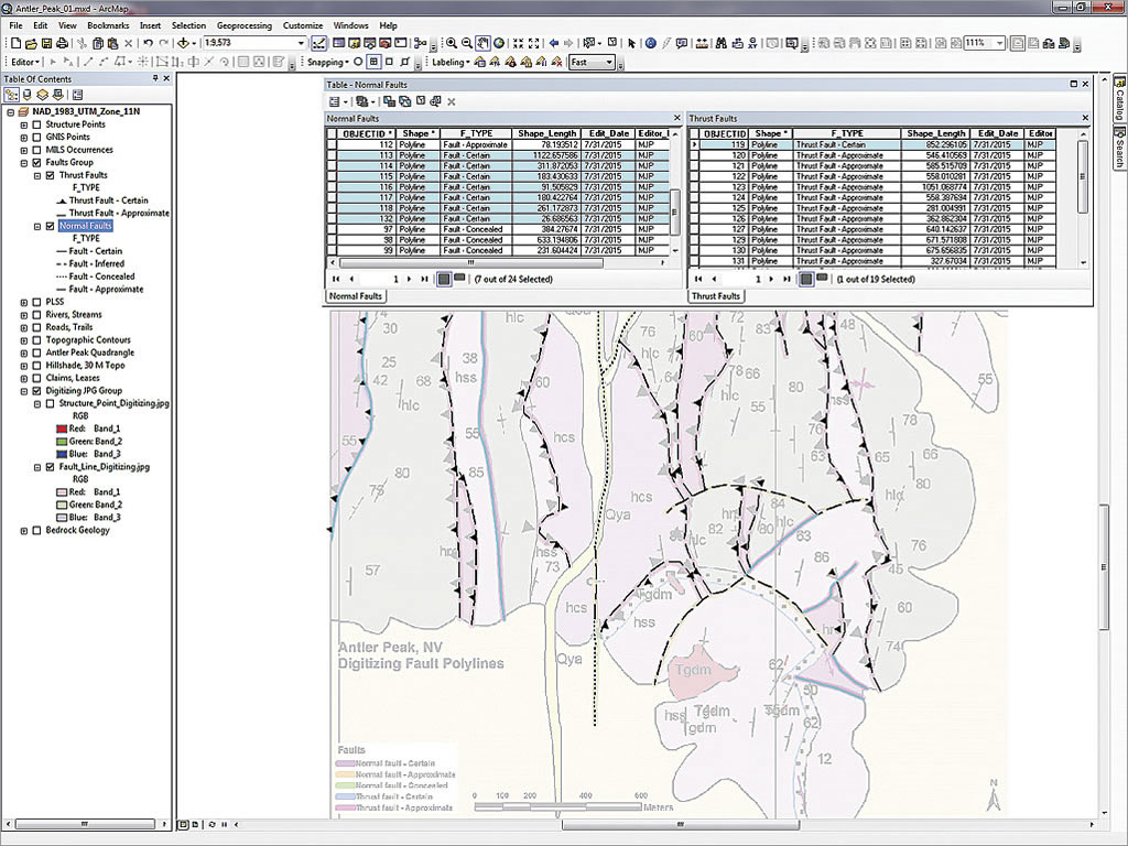
Start ArcMap and open the ArcMap document (MXD) named AntlerPeak01.mxd. It resembles the end product of the previous exercise, which also used data from Antler Peak, Nevada. Note that the frame scale is 1:50,000 and no reference scale has been set. The table of contents (TOC) contains layers in the Faults Group, but these layers are now empty. As part of this exercise, new fault datasets showing much more detail will be created.
Before adding data and resizing your map, complete the map document properties for this MXD and set a default geodatabase.
- From the Standard menu, choose File > Map Document Properties. In the Properties dialog box, fill in the text boxes and set the Default Geodatabase to\GDBFiles\UTM83Z11\Antler_Peak.gdb. Save the map. (Because this project resides in a new folder, data and projects from previous Battle Mountain exercises are unaffected).
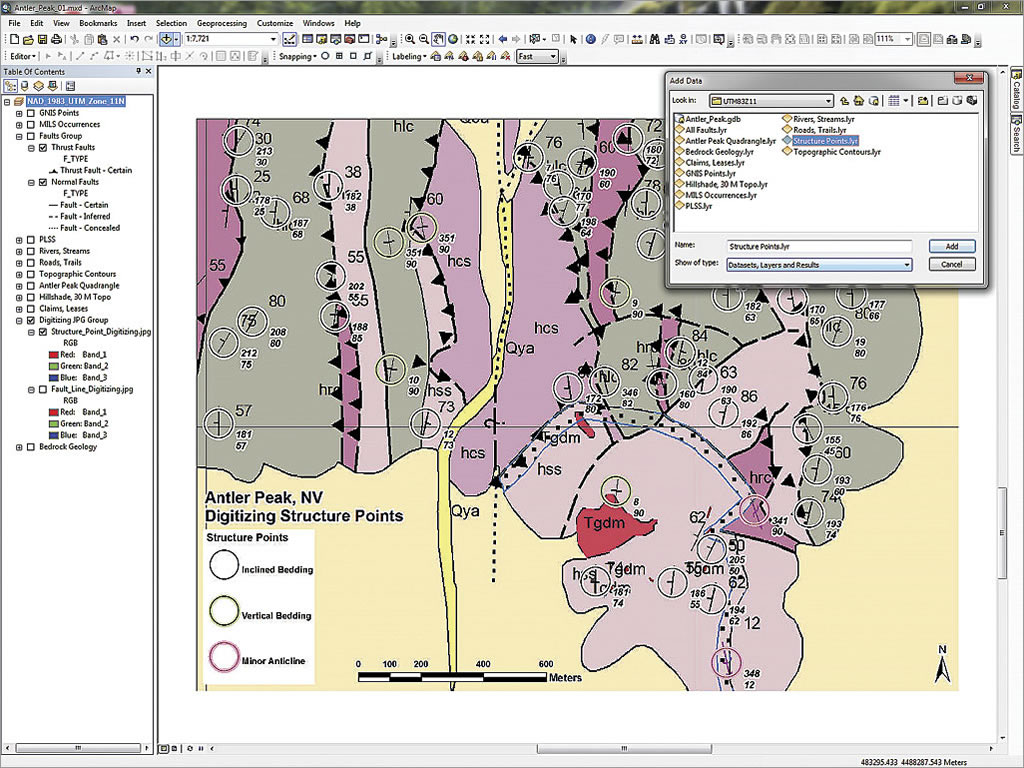
- Load the scanned reference maps for digitizing by navigating to \Battle_Mountain09\JPGFiles\UTM83Z11\ and locating Fault_Line_Digitizing.jpg and Structure_Point_Digitizing.jpg. Add them to the map.
- These rasters are already georeferenced and should appear in the southern portion of the map extent. In the TOC, create a group called Digitizing JPG Group, place Structure_Point_Digitizing.jpg above Fault_Line_Digitizing.jpg, and move the group to the bottom of the TOC, just above Bedrock Geology.
- Turn off all layers except the Digitizing JPG Group and Faults Group. Leave the Faults Group legends expanded and zoom to the Digitizing JPG Group. The data frame scale should be approximately 1:8,467.
- To make map symbols easier to see, choose Data Frame Properties > General and set the reference scale for the data frame to 1:16,000. Verify that the Maplex Label Engine is being used for label placement. Close Data Frame Properties and save the map.
Understanding Strike and Dip
Study the Structure_Point_Digitizing.jpg graphic. It shows many thrust faults and steeply dipping sedimentary rocks. Since compression occurred from the west, many of the linear thrust boundaries trend north to south. Most tilted sedimentary rocks also strike north to south, often dipping steeply toward their western source.
Unless the fault has been completely overturned, the triangular symbols on the thrust faults always point in the direction that the rocks came from. Strike and dip symbols show the alignment of tilted beds in the earth’s broadly curved plane. The short perpendicular barb shows the direction of dip perpendicular to strike. The large black numbers show the posted angle of dip, measured from the horizon. The smaller stacked number pair, located southeast of each point, lists the strike azimuth and inclination (or dip) angle. These pairs will be entered as values for Azimuth and Inclination when digitizing the 50 circled symbols included in this training set.
Loading a Structure Point Template
To expedite this lesson, a Layer file template for the structure points was included in the sample dataset.
- Navigate to \Antler_Peak\GDBFiles\UTM83Z11 and add the Structure Points.lyr. If the link to the data source is broken, relink it to the GeoPoints feature class in Antler_Peak.gdb.
- In the TOC, open Structure Points properties and click the Symbology tab to study its symbology. The three symbols used match US Geological Survey standards for 24,000-scale geologic mapping and are part of the Esri Geology 24K Style set. Structure Points.lyr already assigned point symbols with preset rotations. Later in the tutorial, you will learn to quickly search for missing fault symbology.
- Click the Advanced button, then select Rotation… to look at the symbols’ rotational properties. Each digitized point will soon display its Dip value to allow data entry to be checked visually. Close the Layer Properties dialog box.
- Right-click Structure Points.lyr, open its attribute table, and confirm that it is empty. Notice the fields include Azimuth, Inclination, Label, Edit_Date, and Editor_Initials. These fields will be populated as the points are digitized. Close the table and save the map.
Editing the Template
- This is a good time to open the Editing, Snapping, and Labeling toolbars, so choose Customize > Toolbars to open them.
- To begin editing, right-click Structure Points.lyr in the TOC and choose Edit Features > Start Editing.
- Click the Editing toolbar drop-down and choose Editing Windows > Create Features. Dock this pane on the right side of ArcMap.
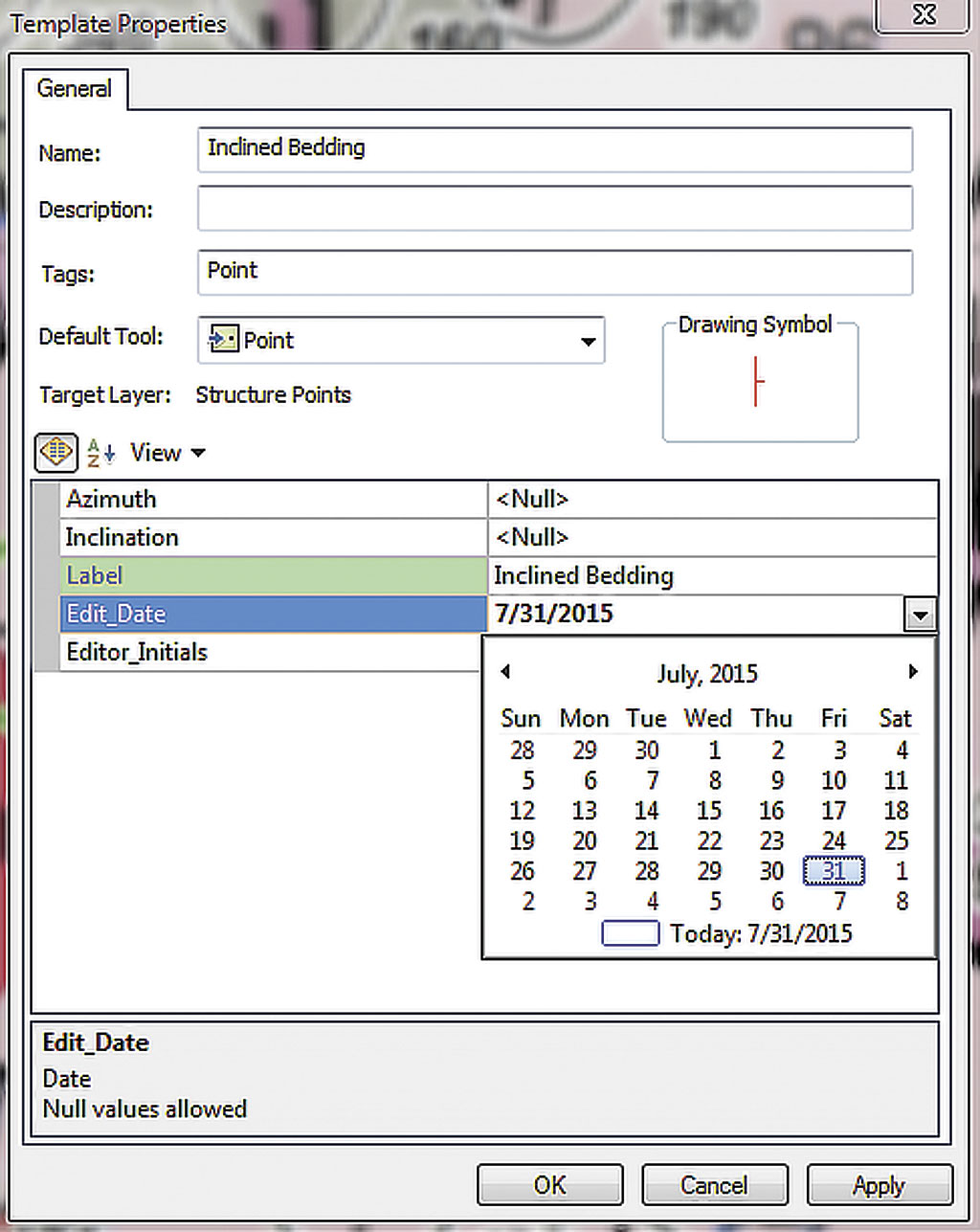
- You should see a prebuilt Structure Points template. In the template, right-click Inclined Bedding and choose Properties.
- Notice that Label is already filled in. Click the blank line next to Edit_Date and select today’s date from the calendar. Make sure you update this field to the current date every time this template is edited. Type your initials in Editor_Initials. Click Apply, then OK.
- Repeat this process for Vertical Bedding and Minor Anticline. Since Inclination for Vertical Bedding is always 90, you may enter it too. Save the map to preserve these updates before digitizing.
Digitizing Points
To digitize two Minor Anticline points, zoom to the southeast corner of the extent and find two magenta arrow symbols inside two magenta circles. Set the data frame reference scale to 1:16,000.
- In the Create Features window, select Minor Anticline. Under Construction Tools, choose Point. Hover your cursor over the map and watch for the downward pointing symbol.
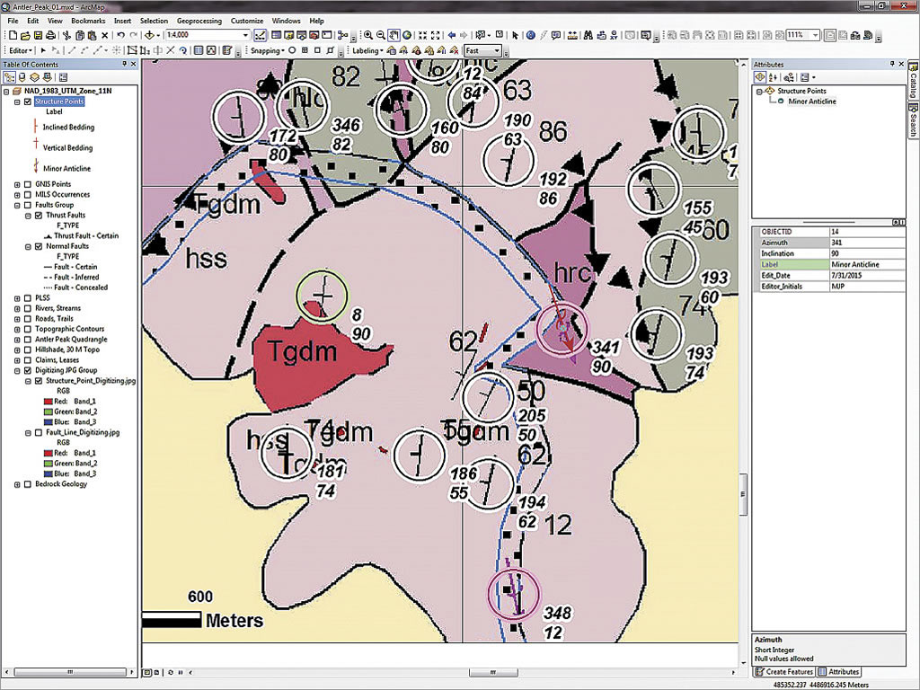
- Click in the center of the most southern magenta circle to drop the first point. On the Editor toolbar, click the Attributes tool.
- Locate the stacked numbers immediately southeast of the magenta target circle and type the upper number in the Azimuth field and the lower number in the Inclination field. Hit Enter and watch the symbol rotate. The Inclination label will also appear.
- Repeat the process for the other Minor Anticline point shown inside a magenta circle. Because the Inclination for this point is 90, the label does not appear because vertical dip values are not displayed. Save your edits.
- Close the Minor Anticline template and select Vertical Bedding and the Point construction tool.
- Locate a green circle and click inside it. An inclined bedding symbol has replaced your regular mouse cursor. Use the graphic underneath as a guide to determine where to click and place the symbol.
- In the Attributes window, enter the appropriate azimuth and check the symbol. Pan or zoom around the map, looking for other green circles. Drop points inside each one and enter the appropriate azimuth. (Hint: Hit the Tab key to assign the last field entry.)
- Save the map to save these edits.
- There are 42 Inclined Bedding points. You do not have to enter all of them, but do enough of them to get a feeling for the method. Pan/Zoom to an area with multiple black circles. Select Inclined Bedding, then Point, and click inside any black circle.
- Enter azimuth and inclination values and check that the inclination angle shown in red is correct.
- After editing several points, you will find the sweet spot to drop each new point.
- If you do not like a point’s location, rotation, or label, you can edit the point and its attributes or delete it and start over.
Use the stacked numbers to the southeast of each point to enter Azimuth and Inclination. In the real world, you might enter these values directly from your field notes after you place each point. Remember that when looking in the strike direction, the dip direction is always to the right of the strike bar. If the dip appears to be in the wrong direction, add/subtract 180 to/from the azimuth value.
If an Inclination label obscures a new point, you can temporarily turn labels off or change the reference scale. When you have digitized most or all points, save the edits and stop editing. Open the Structure Points attribute table to see the values that have been added. Save the map.
Adding a New Fault Type
The next step will be to digitize five faults: three normal faults and two thrust faults. Fault types are color coded, as shown in the JPG legend. Since there are only a few normal faults, start with them.
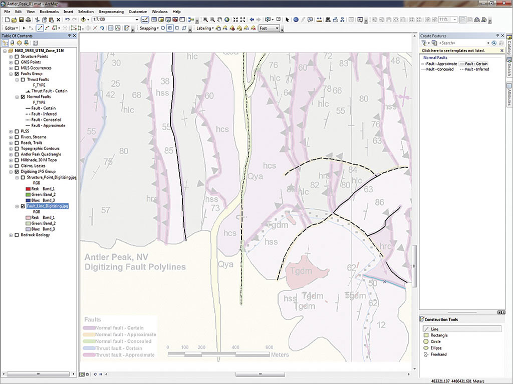
- In the TOC, turn off Structure_Points_Digitizing.jpg and turn on Fault_Line_Digitizing.jpg. Zoom to the Digitizing JPG Group.
- Make Faults Group and its Normal Faults layer visible. Notice that the Normal Faults legend does not include a Fault—Approximate type.
- To add “Fault—Approximate” type, right-click Normal Faults and select Edit Features > Define New Types of Features.
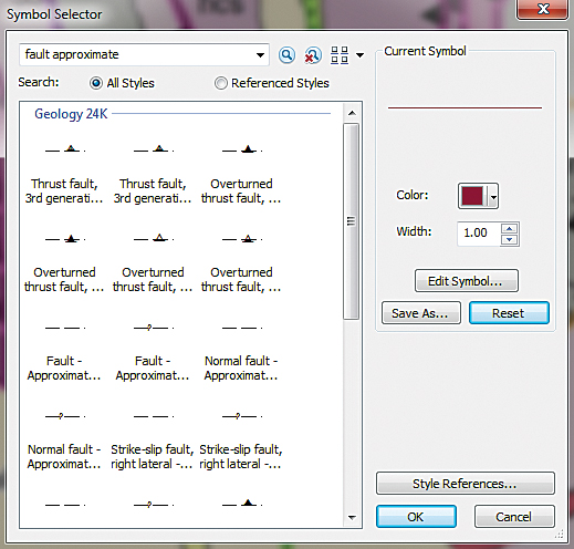
- In the Define New Feature Type window, type “Fault—Approximate” in the Name and Description windows. Click the Change Symbol button and type “Fault—Approximate” in the Search window, searching All Styles.
- Scroll through the results and select the first Normal Fault—Approximate located. Click OK and Next to continue. When prompted, enter today’s date and your initials in the appropriate fields. Click Finish to add the new type. Do not define additional feature types. Confirm that the new type appears in the Normal Faults legend.
- Right-click Normal Faults and select Edit Features > Start Editing. Reopen the Create Features window if needed. Notice that Normal Faults has an editing template with only one member. Delete it.
- At the top of the Create Features window, locate and click the Organize Templates button. In the Organize Feature Templates window, highlight Normal Faults and select New Template.
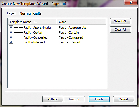
- In the Create New Template wizard, select Normal Faults and click Next. Select all types and click Finish, then Close.
- There should be four fault types, including Fault—Approximate. Open Properties for each type and enter today’s date and your initials. Save the map.
Updating Normal Faults
Before digitizing, set the snapping parameters. In the Snapping toolbar, select only End Snapping. Select Fault—Certain type, followed by Point.
- Start in the south project area and digitize a single green line. Zoom and pan. If you come to any highlighted fault junction, finish the current sketch and start a new one. Continue until you digitize all Fault—Certain lines.
- If a new fault shares an endpoint with a previous segment, snap to the existing feature’s endpoint. Since there is no directional information on normal fault movement, digitizing direction is not critical, although it might be modified later. However, remember that the symbology for thrust faults is directional!
- Next, digitize all Fault—Approximate (orange) lines and all Fault—Certain (purple) lines. Remember to finish each segment at junctions with Normal and Thrust Faults.
- When you have finished digitizing all normal faults, zoom to the extent and increase the transparency of Fault_Line_Digitizing.jpg. Check the accuracy and symbology of all normal faults. If lines are not as detailed as you want, you may edit them interactively. Be sure to make normal faults selectable.
- When finished, save your edits and the map.
Digitizing Thrust Faults
- Now to digitize thrust faults. In the TOC, make the thrust fault layers visible along with normal faults (that will be used for snapping).
- The Thrust Fault—Approximate type must be added first. Right-click Thrust Faults, select Properties, and open the Symbology tab. Click the Add Values button and type “Thrust Fault—Approximate” in the New Value window. Click Add to List and OK.
- Type “Thrust Fault—Approximate” in the Label field and click the new Symbol patch. In the Symbol Selector, search for thrust fault approximate and select Thrust fault, First generation—Approximately located.
- The next step is to complete the Thrust Fault feature template and begin digitizing. In the TOC, right-click Thrust Faults and select Edit Features > Start Editing.
- Reopen the Create Features window if necessary and make sure it contains the Thrust Faults template. Update the Edit_Date and Editor_Initials field in the template for Thrust Fault—Approximate and Thrust Fault—Certain. If the template is incomplete or missing sections, delete it and create a new template using the same steps used to create the Fault—Approximate template.
- Remember from the previous exercise in the summer 2015 issue of ArcUser that thrust fault symbology includes a directional component. Because these rocks moved from the west, the triangles should be pointing toward California. Matching the map, digitize all Thrust Faults—Certain and Thrust Faults—Approximate in that direction, placing JPG triangles on the left side of the line.
- Continue digitizing all thrust faults, snapping to previous endpoints wherever possible. If you forgot to split an earlier line, you are still editing all faults, so you may split (or join) them as needed.
- When you are finished, save edits and review your work. Make Fault_Line_Digitizing.jpg partially transparent to guide your visual inspection. Open both fault tables and confirm that attributes are properly filled.
- Save the map one final time. The exercise is done.
Summary
Was this quite a task, or was it really not that difficult? Did you find that as you practiced and experimented with templates that snapping, editing tables, changing scale, adjusting labels, and heads-up digitizing became easier? Consistently updating the editing date and editor’s initials is an invaluable practice.
Acknowledgments
Thanks to the Battle Mountain data providers and my earth sciences followers. Special thanks to my editor who still keeps me heading in the right direction. Happy editing.