Time is an important dimension in many types of geospatial visualizations and analyses. The temporal aspect adds when to the where and what of data and allows us to see change.
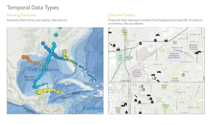
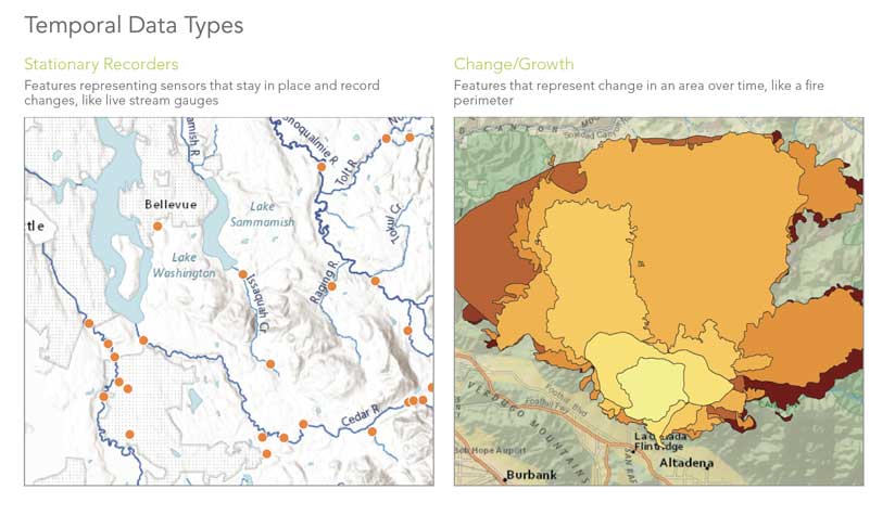
With temporal data, you can analyze and visualize moving things (planes, satellites, storms), events (accidents or crimes), readings that vary over time but originate from stationary sensors (precipitation readings or traffic counts), or the change in the characteristic of a place over time (population change in a census tract or the change in sea surface temperature). Although other cultures have different conceptions of time, we generally think of time as linear and unidirectional. Even events that are cyclic are conceived of as linear (last year, this year, next year) but repeating (winter, spring, summer, fall). ArcGIS treats time in a similar linear fashion.
Time is always relative to something: a clock, an event, or a state. Clock-driven time is synchronized to a specific clock and is an example of regular time data taken at regular intervals. Examples include 15-minute readings from stream gauges and regularly scheduled GPS fixes from animal-tracking devices. Event-driven time is synchronized to an event like dinnertime or before and after a hurricane or flood. State-driven time is synchronized to a change in state; examples include the melting of ice sheets, changes in the economy such as a period of inflation, or the change from one governmental regime to another. Time can be recorded as an instant (a single point in time) or a duration (an interval of time with start and end instants). The interval between recorded time instants can be regular (a 15-minute interval for stream gauges or a decade for a census) or irregular (the incidence of crimes or the change in political boundaries).
Time measurements are either calendar or noncalendar based. An example of calendar time is the Gregorian calendar, which is based on the amount of time it takes the earth to orbit the sun (approximately 365 days) and the earth to rotate on its axis (24 hours). The format can be as simple as year (YYYY) or as complex as decimal fractions of seconds (YYYY/MM/DD hh:mm:ss.s).
Although this is the most widely used calendar in the world today and most people understand it well, it is difficult to compute from because it is not metric or in base 10. There are variations in some measures (such as the number of days in a month) but not in others (there are always 60 minutes in an hour and 60 seconds in a minute).
Noncalendar time is synchronized to a specified time instant. The time instant chosen as the origin and reference point from which time is measured is called an epoch, and time measurement units are counted from the epoch so that the date and time can be specified unambiguously. An example of noncalendar time is the computer system time used in Unix, Java, and Oracle, which reflects the count of seconds since January 1, 1970, which is also 00:00:00 in Coordinated Universal Time (UTC).
GIS Integrates Temporal Data
Time is built into ArcGIS Pro, ArcMap, the ArcGIS Runtimes, and portal so the temporal dimension of geospatial data can be used for analysis, simulation, and modeling across the ArcGIS platform. Geoprocessing tools can be used to manage time-aware data and analyze space-time data. Space-time data can be visualized in ArcGIS Pro, ArcMap, ArcScene, ArcGlobe, and ArcGIS Online.
Supported temporal data types include feature layers, mosaic datasets, Network Common Data Form (netCDF) layers, tables, raster catalogs, tracking layers, streaming layers, network dataset layers with traffic data, and service layers with historical content and updating data feeds. In ArcGIS, time information is stored as attributes (for feature classes and mosaic datasets), or it is stored internally (as with netCDF data).
For feature classes, time is enabled and configured through the Time tab on the feature layer’s properties. For features, the shape and location of each feature may be constant, but attribute values can change over time.
Alternatively, both the shape and location of each feature may change over time. If the shape and location do not change, there are two ways in which the data can be stored: as duplicated features with unique time values or unique features that are related to a table with time values.
An example is a dataset of the 100 largest cities in the United States by decade. In this case, cities might be duplicated each time they are included in the list of 100, or a single set of cities could be related to a table with the decades in which they appear in the list. If the shape or location changes, each feature must be stored along with its time value. An example is a dataset with the burn extents for a wildfire.
Mosaic datasets store rasters that represent change over time. While time is enabled and configured using the mosaic dataset’s properties, the time attribute is stored in the attribute table of the Footprint layer of the mosaic dataset.
NetCDF is a file format for storing multidimensional (x, y, z, t) data in an array with x and y representing space and t representing time. The z dimension stores one or more attributes such as temperature, salinity, pressure, and wind speed. For netCDF feature layers, the layer time is specified using a time dimension or attribute field. For netCDF raster layers, layer time is specified using the time dimension.
Temporal data and information products based on temporal data can be shared in a variety of ways through maps, map layers, packages, and more. These can be viewed as static images or dynamic visualizations, and they can be shared as either paper or other print products or in digital format. Temporal data is increasingly being used in web map layers, web maps, story maps, and other online products.
Best Practices for Managing Temporal Data
How temporal data is stored and managed affects its use by ArcGIS. Use the following best practices to avoid issues.
Whenever possible, store time values in a date-type field for the most efficient query performance and more sophisticated database queries. Date display is only supported for the time extent of AD100 to AD10,000. To work with dates outside this extent, convert your values into a numeric format and use the range slider to visualize the data.
To convert time values stored in a text or numeric field (short, long, float, or double), use the Convert Time Field geoprocessing tool. This tool converts the values to a supported or custom-defined date format and records it in a new date field. For example, “July 9, 2016” in a text field would become “2016/07/09” in a date field with the format YYYY/MM/DD.
Convert time attributes stored in multiple columns to rows using the Transpose Fields geoprocessing tool because ArcGIS works with temporal data in row format. This tool is useful for working with census data, which often uses multiple columns to store temporal attributes.
Daylight saving time is a challenge to work. This is because some areas use it, while others do not; the variations can be in offsets other than a single hour; and the rules and boundaries change frequently. Therefore, it is better to store time attributes in standard time rather than daylight saving time. Index time attributes for faster query performance.
Visualizing Temporal Data
In ArcGIS, visualizing temporal data is a two-step process. First, enable time on a layer and configure the associated time properties, such as specifying the time attribute or attributes, setting the time extent by selecting the first and last time instants to be displayed, and indicating the refresh rate for live feed data. Other settings can also be used, for example, to manage for differing time zones and daylight saving time. Once this step is done, you have created a time-enabled layer.
Second, use the time slider to control visualization of the time-enabled layer by playing, pausing, stepping forward or back, setting the time step (the span between time instants that the data is visible), and more. The time slider control will automatically appear in any map or scene that has time-enabled layers. You can also use the time slider to configure additional settings to control the display of the data in the map.
Analyzing Temporal Data
There are three ways in which temporal data can be analyzed in ArcGIS:
- The data for each time step is analyzed separately, and the individual analysis results are presented as a single layer for a single time step or a set of layers, one for each time step.
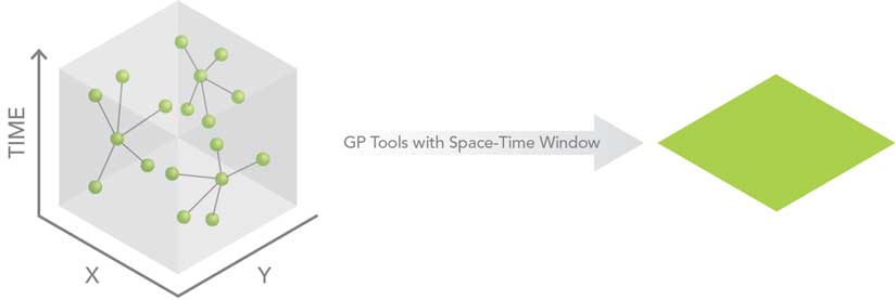
- The data is analyzed using constraints in both space and time, and the results are presented as a single layer.
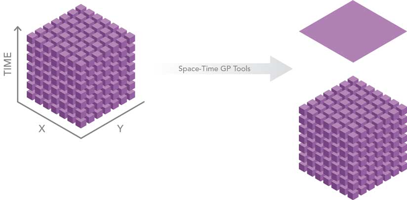
- The data for all time steps is analyzed both spatially and temporally, and the results are summarized in a 2D layer or presented as a 3D layer in which time is displayed in the z dimension.
Taking the first approach, the analysis is dependent on the time step that has been specified, so if yearly data is analyzed by decade, then each result will reflect the analysis of 10 years’ worth of data.
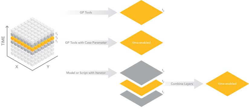
There are three ways in which this type of analysis can be performed. First, all geoprocessing tools honor the time settings for time-enabled layers so only those features that fall temporally within the time extent set in the time slider will be processed. The results are then displayed as a single layer on a map.
Second, with some tools (for example, Mean Center and Directional Distribution), the time attribute can be used as the case field to repeat the analysis for each time step. [The case field is the field in the input used to calculate statistics separately for each unique attribute value.] These results are presented as a single layer, and time can be enabled on the case field, which is copied into the output feature class.
Third, a model or script can be created using an iterator to specify that the analysis should be repeated for each time step. This approach results in separate outputs for each time step. The separate outputs can then be combined (for example, using Merge or Append for feature classes or adding the rasters to a mosaic dataset) so that the final result can be time enabled and visualized using the time slider control.
Certain geoprocessing tools take the second approach to analyzing space-time data. These tools use a spatial weights matrix that defines feature relationships in terms of a Space-Time Window with a specified critical distance and a fixed interval in time. The tools that use this matrix include the Hot Spot Analysis, Cluster and Outlier Analysis, and Grouping Analysis tools.
The Hot Spot Analysis tool creates a map of clusters in both space and time of significantly high (hot) or low (cold) values. The Cluster and Outlier Analysis tool identifies the similarity (as the spatial clustering of either high or low values) or the dissimilarity (as spatial outliers) of features. The Grouping Analysis tool groups features based on feature attributes.
The third approach uses a set of tools in the Space-Time Pattern Mining toolbox and includes the Emerging Hot Spot Analysis, Local Outlier Analysis, and Fill Missing Values tools. The Emerging Hot Spot Analysis tool identifies hot and cold spots and determines if they have a temporal trend (new versus persistent versus historic hot spots). The Local Outlier Analysis tool determines if features have belonged in clusters or been outliers over the entire time extent of the dataset. The Emerging Hot Spot Analysis and Local Outlier Analysis tools require that the data be in a space-time cube format.
The Fill Missing Values tool, located in the Utilities toolset that is designed to be used with the Space-Time Pattern Mining toolbox, replaces missing values with estimates based on spatial neighbors, space-time neighbors, or time-series values.
The two other tools in the Space-Time Pattern Mining toolbox can be used to create the space-time cube depending on whether the input is a set of points or polygons.
The space-time cube can be viewed in either 2D or 3D using the Visualize Space Time cube tools (also found in the Utilities toolset for the Space-Time Pattern Mining toolbox or with an add-in called the Space Time Cube Explorer.
For more traditional time series analysis, you can take advantage of the extensibility of the ArcGIS platform with its capabilities to easily transfer data to open-source analytical software. For example, you can use ArcPy utility functions, such as FeatureClassToNumPyArray, to analyze the data in Python, or the R-ArcGIS Bridge to analyze the data using R.
Sharing Temporal Data and Maps
Temporal maps and data can be shared as packages. Temporal maps can also be shared as a set of exported graphic images, each representing a different time step, or a temporal map series in which a collection of map pages, one for each time step, are built from a single layout. Time-enabled web layers and web maps can also be created. These will automatically be displayed with a configurable time slider control in the ArcGIS Online Map Viewer.
With ArcMap, exporting time-enabled web layers requires the use of a GIS server. With ArcGIS Pro, you can publish hosted feature layers that include temporal data directly to ArcGIS Online. Time for these layers is enabled on the item page for each layer. Mosaic dataset images can be exported from either ArcMap or ArcGIS Pro as an image service—this requires the use of a GIS server.
Animations can be used in ArcGIS to create, edit, and export a temporal visualization. With animations, you can navigate through a display, follow the view along a path, move point features along a path, and visualize time-enabled data from a static or moving camera. Because you can use any combination of these, animating time-enabled data can create intriguing and informative dynamic displays of temporal phenomena.
In ArcGIS Pro, animations can be exported to a video or folder of frames using draft, preset, or custom settings. The draft option exports the animation to an AVI movie for previewing before a final version is created.
The preset options export to commonly requested formats including YouTube, Vimeo, Twitter, Instagram, HD720, HD1080, and GIF. Manual settings for the format, resolution, frames per second, and quality of the video export can be saved as custom presets for a project. Because the options for video export in ArcGIS Pro are so versatile, a best practice is to import your time-enabled ArcMap document into ArcGIS Pro to generate a video.
Conclusion
The ArcGIS platform gives you control over your temporal data from start to finish, allowing you to manage, analyze, and visualize information about space and time in insightful and effective ways. Esri is continually developing tools for using temporal data so you can work with your space-time data.
Thanks to Esri staff Kevin A. Butler and Lauren Scott Griffin for their help ensuring the accuracy of the analysis section of this article.