A space-time cube is a dataset that contains both spatial and temporal data, organized into bins. When visualized in 3D, the bins are stacked on top of each other along the z-axis (the third axis in a 3D coordinate system) to indicate time. Space-time cubes enable you to better understand and analyze spatiotemporal data.
In this tutorial, you’ll use ArcGIS Pro to create and explore a space-time cube layer of homeownership rates in Florida since 2010. Space-time cube layers are created to visualize the contents of space-time cube netCDF (network Common Data Form) files. The space-time cube you’ll use in this tutorial contains United States Census Bureau data from the American Community Survey (ACS).
This tutorial uses ArcGIS Pro 3.6. If you’re using a different version of ArcGIS Pro, you may encounter different functionality and results.
ArcGIS Pro is required—see options for software access.
Create a Project
First, you’ll download the space-time cube netCDF file and create a project in ArcGIS Pro with a 3D scene.
1. Download Florida_Housing.zip.
2. Extract the downloaded zipped folder to a location of your choice, such as your Documents folder.
The Florida_Housing.zip folder contains FloridaHousing.nc. The .nc extension is used for netCDF files, including space-time cubes. The file contains ACS housing and demographic data for Public Use Microdata Areas (PUMAs) in Florida. PUMAs are geographies defined by the United States Census Bureau that contain at least 100,000 residents.
3. Start ArcGIS Pro. If prompted, sign in using your licensed ArcGIS organizational account.
You’ll create a project with a scene. Scenes display data in 3D. Space-time cube layers are used for 3D visualization of spatiotemporal data, so it’s best to use a scene to work with them.
4. Under New Project, click Local Scene.

5. In the New Project window, for Name, type “Florida Housing Trends”. Click OK. The project is now created and includes a scene with a default extent.
Before you make the space-time cube layer, you’ll turn off the scene’s default elevation surface. Because space-time cube layers use the z-axis (elevation) to represent time, it’s best to hide any 3D layers that may interfere with the visibility of the space-time cube layer.
6. In the Contents pane, under Elevation Surfaces, uncheck WorldElevation3D/Terrain3D and, if necessary, any other elevation surfaces.

Make the Space-Time Cube Layer
Next, you’ll run a geoprocessing tool to create a space-time cube layer using the space-time cube netCDF file you downloaded.
1. On the ribbon, click the Map In the Layer group, click the Add Data drop-down menu.

2. In the drop-down menu, click Space Time Cube Layer.

Note: If you don’t see the Space Time Cube Layer option, make sure the active view is a scene, not a map. The highlighted tab above the view indicates what the active view is.
The Geoprocessing pane appears, showing the Make Space Time Cube Layer tool.
3. For the Input Space Time Cube parameter, click the Browse button.

4. In the Input Space Time Cube window, browse to the location of the Florida_Housing folder you extracted. Choose nc and click OK.
The file is added to the tool parameters.
5. For Output Feature Class (Layer Source), delete the existing text and type “Florida_Housing_STC” (STC is short for space-time cube).
When you added the netCDF file, the Variables parameter became populated with all variables associated with the space-time cube. Many of these variables contain census information that is not relevant to homeownership rates, so you don’t need them for this tutorial. You’ll select one relevant variable to include in the space-time cube layer.
6. For Variables, click the Reset All variables are deselected.

In the list of variables, check the box for HOMEOWNERSHIPRATE (homeownership rate).

You’ll leave the output geometry type as points. Points will appear as 3D bins in the scene and, in this instance, have better rendering performance.
7. Click Run.
The tool runs. When it finishes, the space-time cube layer is added to the scene, showing cube-shaped bins across Florida. The space-time cube layer is only a visual representation of the actual space-time cube, which is in the netCDF file.

Before you explore the scene, you’ll investigate the details of the tool results to learn more about the space-time cube layer.
9. At the bottom of the Geoprocessing pane, click View Details.

A details window appears with information about the tool results.
10. If necessary, scroll to the top of the Space Time Cube Layer Characteristics section.
The space-time cube layer’s data ranges from 2010 to 2023. The time step interval is 1 year, meaning each bin on the scene represents a year of data.

11. Close the details window.
Navigate the Scene
Next, you’ll navigate the scene to see what you can learn about the space-time cube layer.
1. Use your mouse or the navigation controls to pan, tilt, and zoom in to the scene until you can see an oblique view of the entire layer.
Tip: To learn more about navigating a scene, read Navigation in 3D.

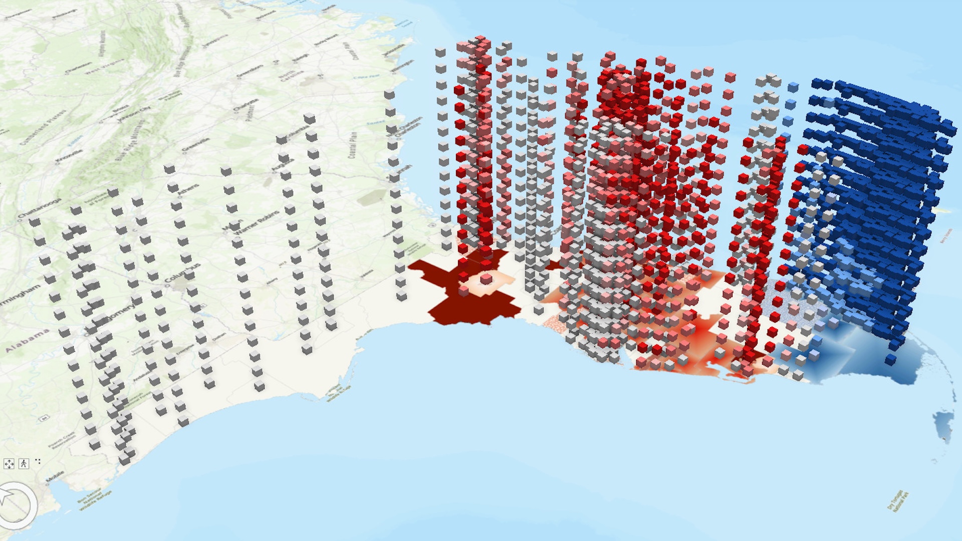
Each column of the space-time cube layer represents a location. In this case, each location is a PUMA. Each bin (cube) represents a single time step; as you saw in the details window, each time step is one year’s data.
The bin closest to the ground is the earliest time step, 2010. Each subsequent bin represents the next year, ending with the bin at the top, which represents 2023. Each column contains 14 bins, representing the 14 years between 2010 and 2023.
The bins are symbolized by the variable value. The variable value is listed in the Contents pane, above the layer’s legend.

In this case, the variable value is the homeownership rate variable. Darker bins represent higher homeownership rates. Based on the legend, the bin with the lowest rate has about 13.9 percent homeownership, while the bin with the highest has about 89.1 percent homeownership.
From this default visualization, you can already see some spatial and temporal trends in the data, helping you discover how homeownership rates change over time and space.
2. Pan, tilt, and zoom in to the scene until you can clearly see the southernmost column of bins.
This column has medium-colored bins for the first 13 bins. The final bin, at the top, is darker. This pattern indicates that this area has recently experienced an increase in homeownership rate. The pattern is temporal because all the bins in this column represent the same location, just at different times.

3. Pan, tilt, and zoom in to the scene until you can see the cluster of columns around the city of Jacksonville, located in the northeastern part of Florida.

Near the center of Jacksonville, there is a pattern of lighter-colored bins, indicating low homeownership. However, the areas outside of Jacksonville have darker-colored bins, indicating high homeownership. This pattern is primarily spatial; while there is some difference in rates within the same column, the biggest differences are from column to column.
4. In the Contents pane, right-click Florida_Housing_STC and choose Zoom To Layer. You return to the full extent of the layer.

5. On the Quick Access Toolbar, click the Save Project button. You can also save the project using the keyboard shortcut Ctrl+S.

In this tutorial, you created a space-time cube layer from a space-time cube netCDF file and performed a basic exploration of its data showing homeownership rates in Florida from 2010 to 2023.
Visit the Esri tutorial gallery to explore additional topics and find other step-by-step workflows on a variety of products.