Enabling communities around the world with on-demand urban heat mapping.

According to the United States Environmental Protection Agency (EPA), heat islands are urbanized areas that experience higher temperatures than outlying areas. Structures such as buildings, roads, and other infrastructure absorb and re-emit the sun’s heat more than natural landscapes such as forests and water bodies. Urban areas, where these structures are highly concentrated and greenery is limited, become “islands” of higher temperatures relative to outlying areas. These heat islands can have significant impacts on human health and energy consumption.

Mapping heat islands aids in understanding impacts and creating mitigation strategies. However, with variable data sources and methodologies to consider, this can be a complex undertaking. This article is focused on intra-urban heat islands, mapping the variability of surface heat intensity within a defined urban area extent. Furthermore, our goal is to provide a simple, cost effective, and repeatable process for anyone, anywhere, to begin measuring and analyzing urban heat. This is reflected in the methodology and data source selected.

Jointly managed by NASA and the USGS, Landsat is the longest running spaceborne earth imaging and observation program in history. Landsat Level-2 science products provide global multispectral imagery from 1982 to present, including a derived Surface Temperature product.

ArcGIS Living Atlas of the World enables access to the entire Landsat Level-2 archive as a single imagery layer optimized for analysis. This article provides a step-by-step tutorial for using Landsat imagery from Living Atlas, and analysis tools in ArcGIS Online, to perform analysis and map surface intra-urban heat islands (SIUHI) for urban areas around the world.

Table of Contents

• System Requirements
• Prepare a web map for analysis
• Analysis Part 1: Data Aggregation
• Analysis Part 2: Zonal Mean
• Analysis Part 3: Surface Heat Index
• Assess the results

System Requirements

• An ArcGIS Online organizational account with credits*
• A minimum of a Professional User Type with a Publisher role.
• Imagery layers optimized for analysis capability**

*This tutorial consumes a total of approximately 5 credits. Credit usage will vary based on the temporal and geographic extent.

**Living Atlas imagery layers optimized for analysis provide scalability for larger and more diverse workflows. See ArcGIS Living Atlas ready-to-use imagery layers for analysis for more information including how to enable the imagery layers optimized for analysis capability.

Prepare a web map for analysis

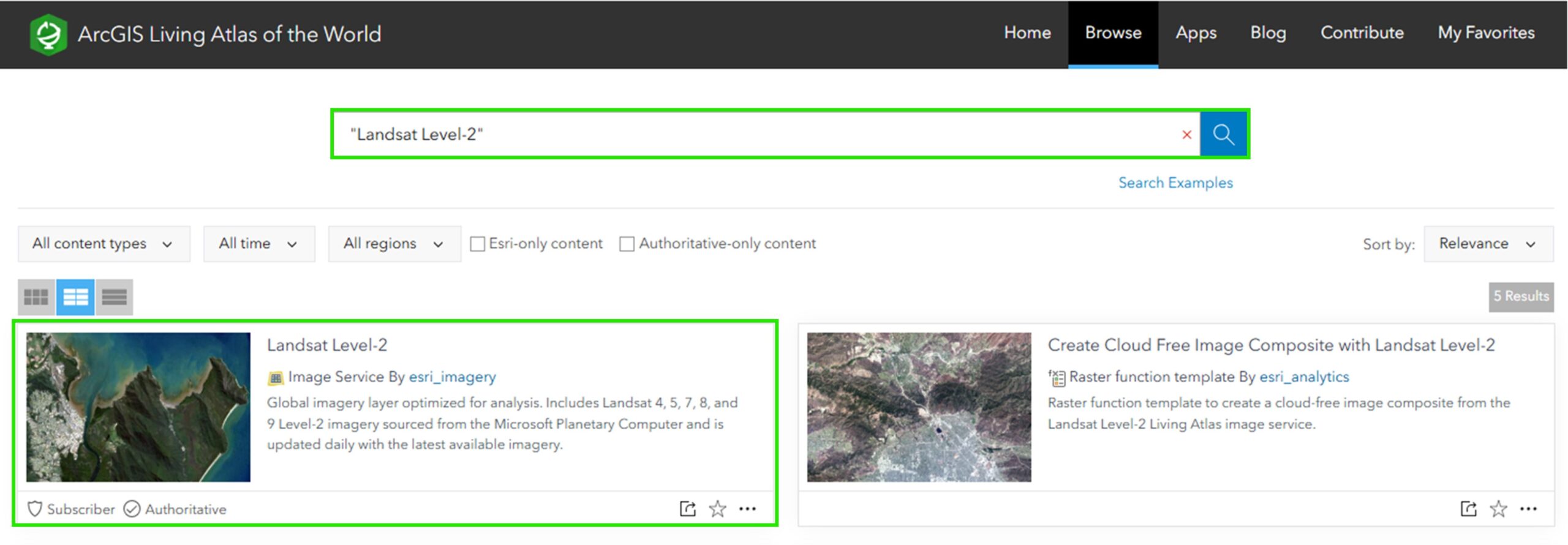
Step 1: Go to the ArcGIS Living Atlas of the World website, enter “Landsat Level-2” in the search bar, and click search. Find the Landsat Level-2 item and click the thumbnail to View item details.

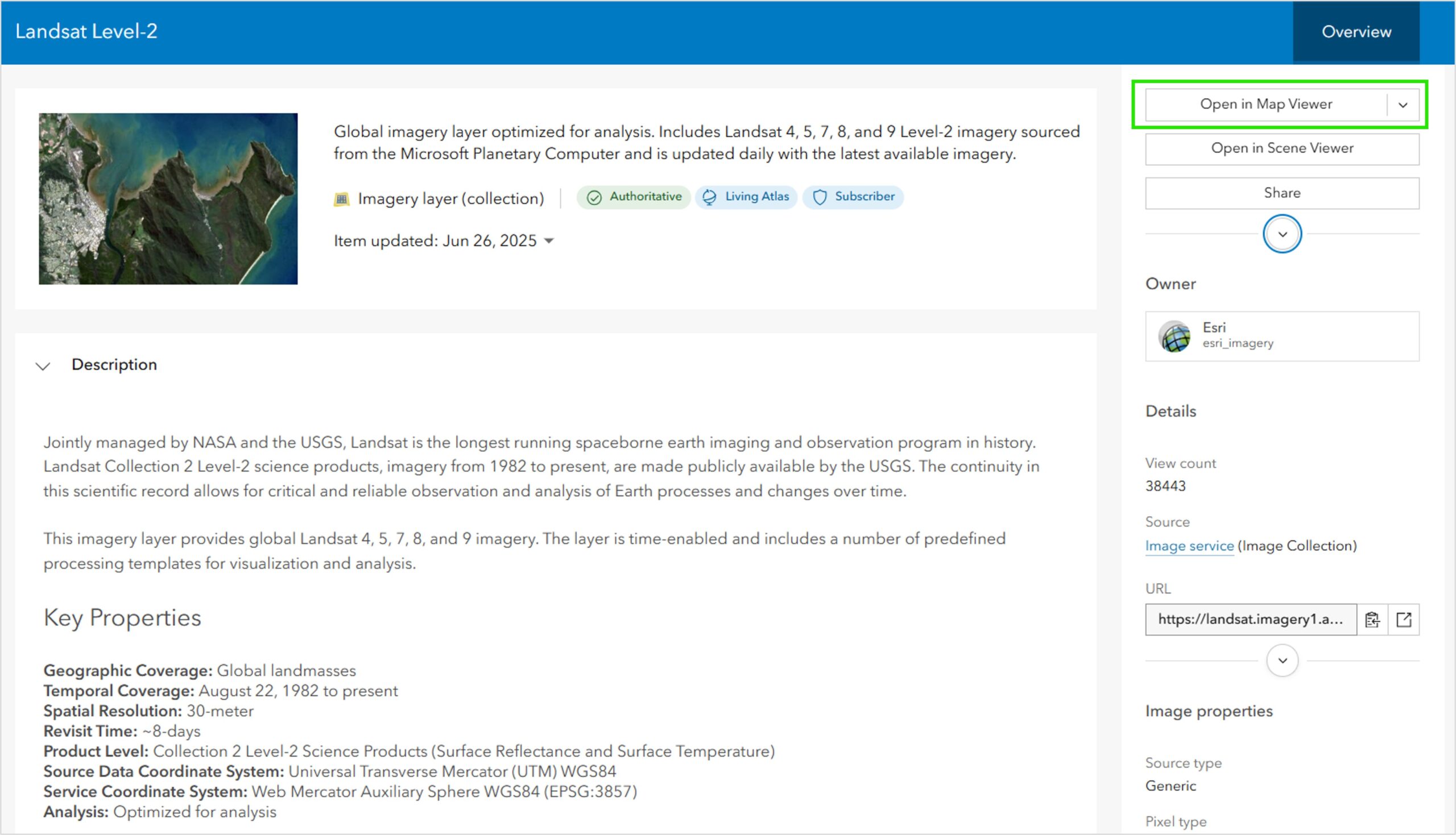
Step 2: All of the details of what this imagery layer provides can be found on this item page, including key properties, available spectral bands, and more. When you are ready to proceed, click Open in Map Viewer.

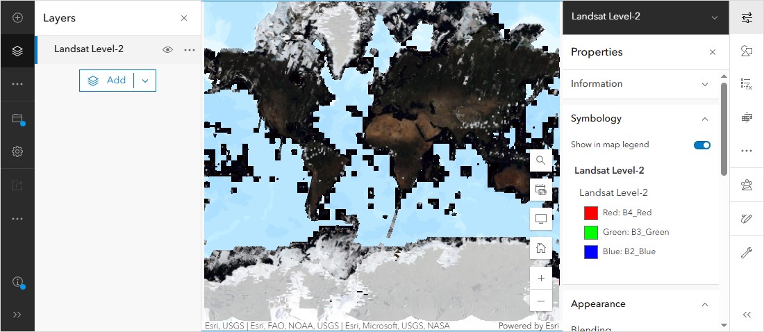
The Landsat imagery layer should now be displayed in Map Viewer. The layer loads with a default “Natural Color” (RGB) rendering.

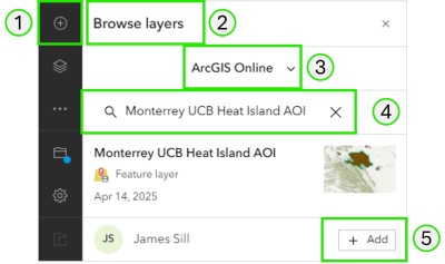
Step 3: Next, a polygon feature will be added to the map to define the area of interest (AOI) and constrain the processing extent for analysis. For this example, we will focus on the city of Monterrey, Mexico.

1. Select Add Layer.
2. Select Browse Layers.
3. Select ArcGIS Online.
4. Enter “Monterrey GHS-UCDB Heat Island AOI” into the search dialogue and click search.
5. Click Add to add the layer to the map.

Step 4: Next, you will load three Raster Function Template (RFT) items into the map, starting with Part 1 of 3. A raster function template is essentially a processing model where multiple raster functions are sequentially chained together to execute a set of commands.

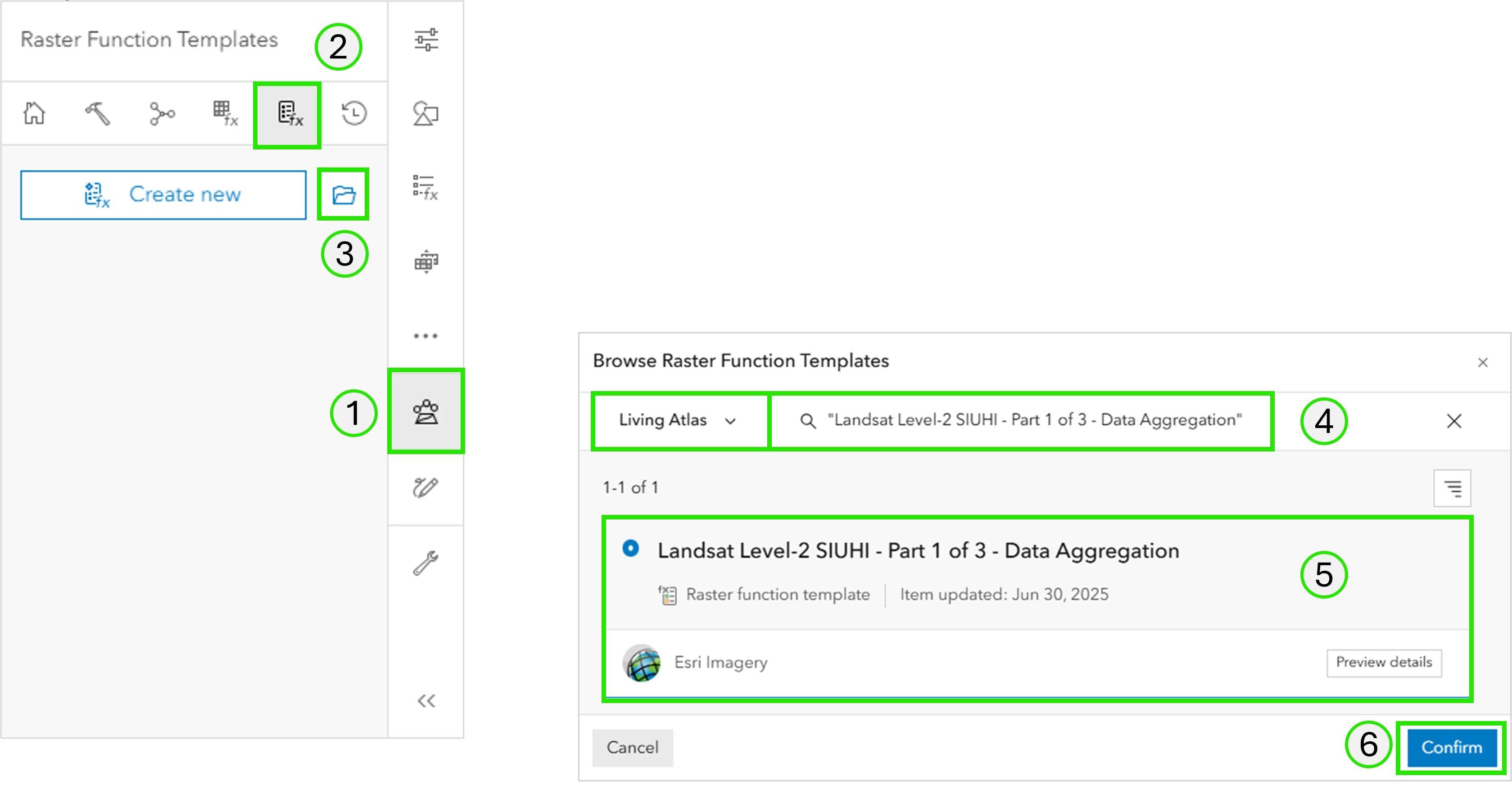
1. Click Analysis on the right side tool bar.
2. Click Raster Function Templates within the Analysis panel.
3. Click Browse Raster Function Templates to open the Browse panel.
4. From the Browse panel, select Living Atlas from the drop down list.
5. In the search bar, enter and search for “Landsat Level-2 SIUHI – Part 1 of 3 – Data Aggregation“.
6. Select the Data Aggregation RFT and click Confirm.

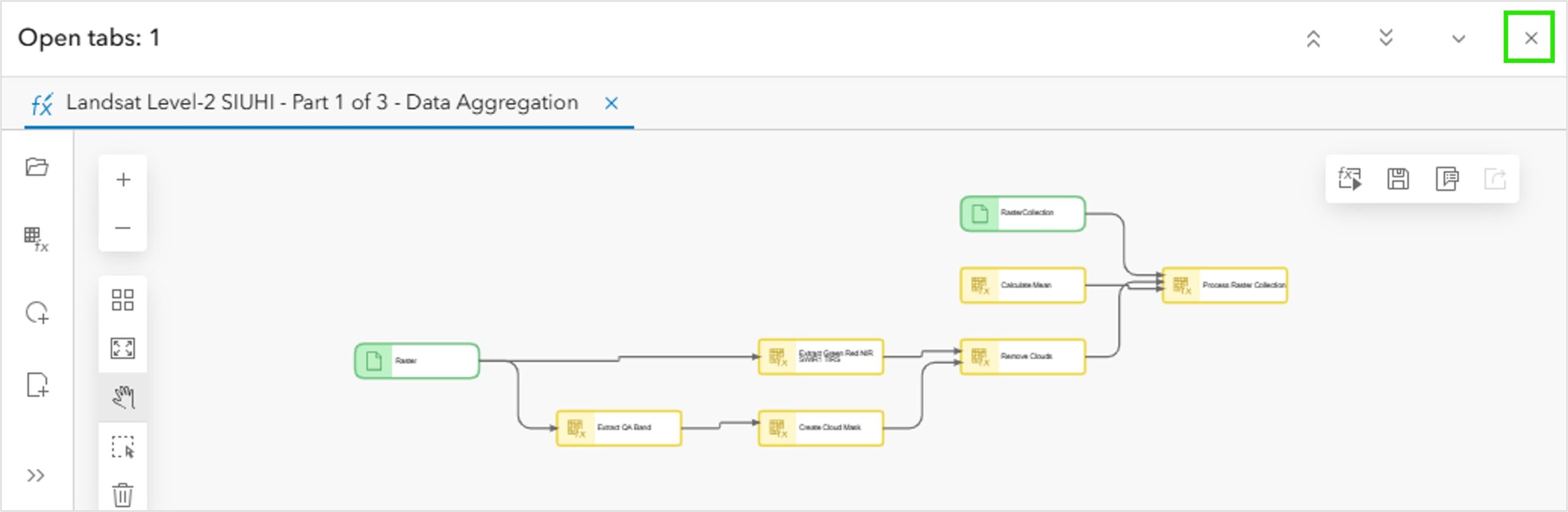
Step 5:  The chain of processing steps within the selected RFT is now displayed in the Edit panel. However, the selected RFT is ready-to-use, so no editing is required. Close the edit panel.

Step 6: Next, you will load the other two RFT’s, Part 2 and Part 3, into your map. Repeat steps 4 and 5 for “Landsat Level-2 SIUHI – Part 2 of 3 – Zonal Mean” and “Landsat Level-2 SIUHI – Part 3 of 3 – Surface Heat Index“.

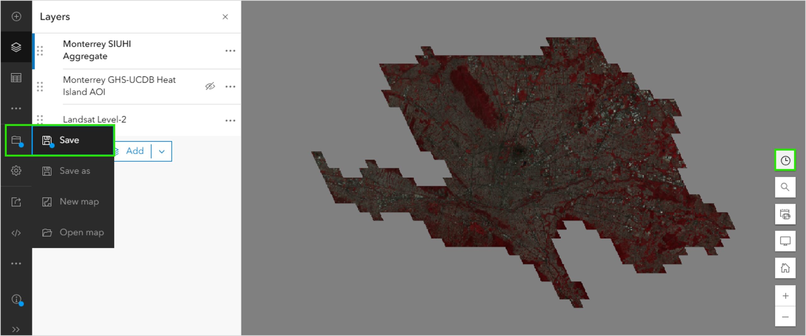
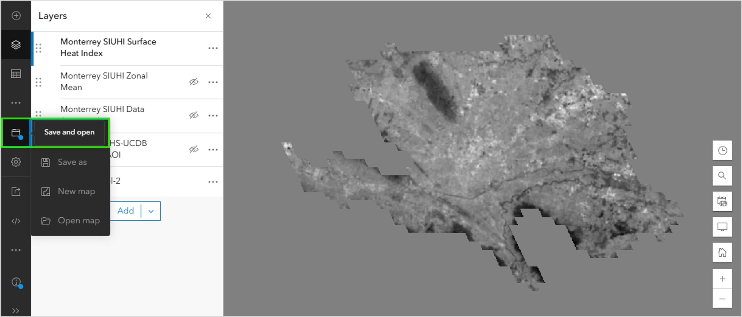
Step 7:  With all three RFT’s, the Landsat Level-2 imagery layer, and the Monterrey AOI successfully loaded into the map, click Save and Save As to save the project as a Web Map item in your ArcGIS Online account named “Monterrey, MX SIUHI“. You are now ready for  Analysis Part 1.

Analysis Part 1: Data Aggregation

The following is a summary of the processing steps involved with the Data Aggregation RFT:

• A spatiotemporal selection of Landsat scenes.
• Band extraction: Green (Band 3), Red (Band 4), SWIR1 (Band 6), Near Infrared (Band 5), Surface Temperature in degrees Kelvin (Band 8), and the QA Band (Band 9).
• A statistical mean calculation of cloud-free* overlapping pixels for each band.

The output produced is a seasonal mean raster containing the five bands required for the SUHI calculation. Note, the QA band is extracted and used only for cloud masking purposes and is not persisted in the mean aggregate output.

Step1:  In the web map created in the first section, set the imagery layer Processing Template to None:

1. Click on Landsat Level-2 from the contents pane to activate the right hand tool bar for that layer.
2. Click on Processing Templates to display the full list of available templates.
3. Scroll to the bottom of the list and select None.
4. Click Done.

Setting the default template to None exposes all the available Landsat Level-2 bands for analysis but results in a solid grey display of the imagery.

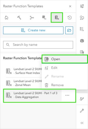
Step 2: Open the first RFT.

1. Under Analysis, open the Raster Function Templates panel.
2. Click the three dots on Landsat Level-2 SIUHI – Part 1 of 3 – Data Aggregation.
3. Select Open.

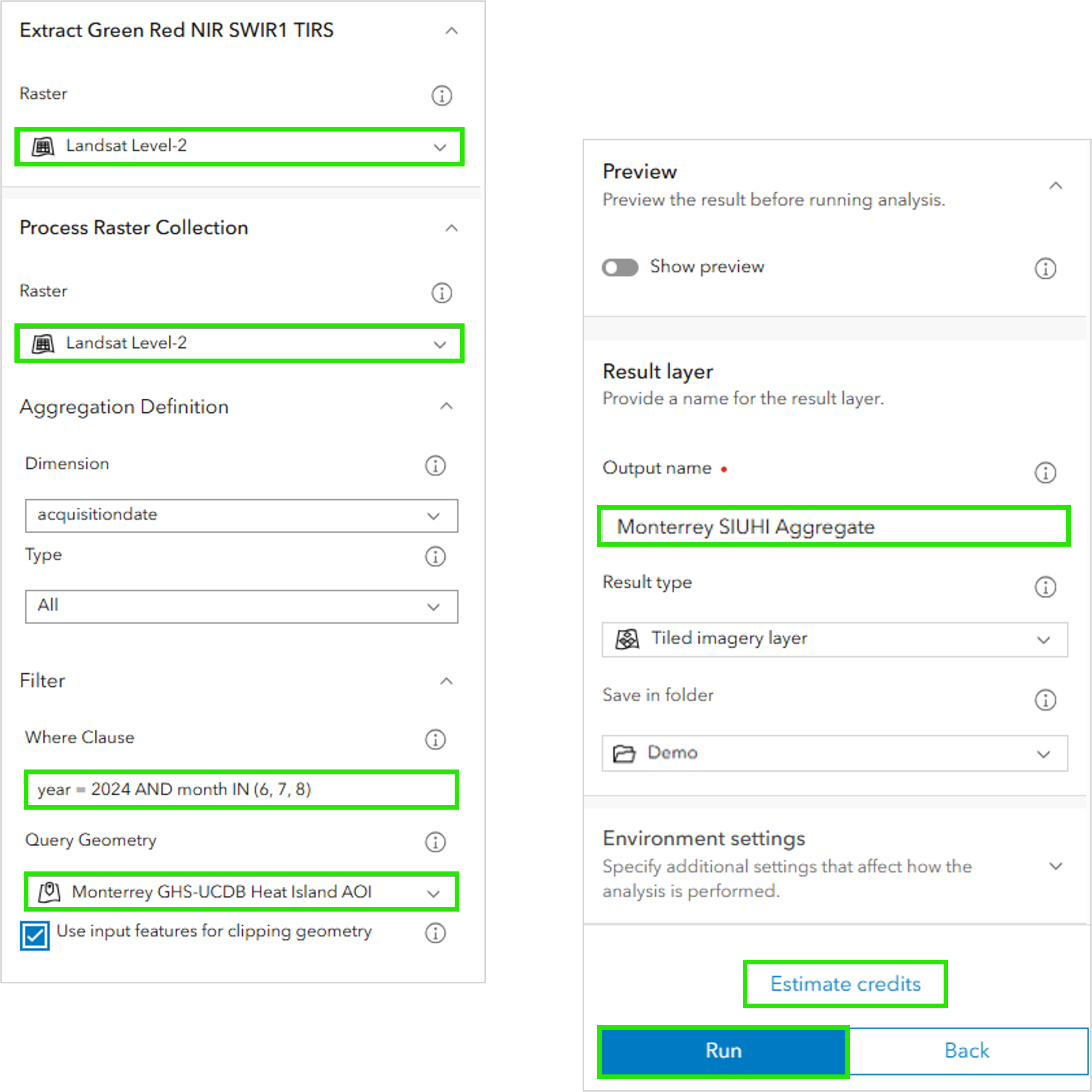
Step 3:  With the input parameters panel now open, enter the required information and run the RFT:

1. Select Landsat Level-2 as the input raster.
2. Enter “year = 2024 AND month IN (6, 7, 8)” as the input Where Clause to constrain the aggregation to images acquired in June, July, and August of 2024.
3. Select Monterrey GHS-UCDB Heat Island AOI as the input Query Geometry and select the option to Use input features for clipping geometry. This will further constrain the aggregation to images intersecting the AOI.
4. Enter an Output name for the output aggregate hosted imagery layer, “Monterrey SIUHI Data Aggregation“. The output will be stored in your ArcGIS Online organization and used as input to the next step.
5. Clicking Estimate Credits will provide an estimate of how many credits will be consumed by the analysis job. Estimating credits is recommended but not required to run the analysis. A larger analysis job (larger area or longer time span) will require more credits.
6. Click Run to begin processing.

NOTE: You can click History to see job history as well as the processing status of a current job.

Step 4: The result of Part 1 – Data Aggregation is a five-band seasonal mean imagery layer clipped to the input AOI boundary. When processing completes, the resulting hosted imagery layer is saved to your organization and displayed in your map. Click the clock icon to turn off the time slider and click Save to save your map. You are now ready for Analysis Part 2: Zonal Mean.

*This workflow provides a simple streamlined way to analyze a collection of images intersecting an area of interest for a specified period of time. The process leverages the cloud mask provided with Landsat Level-2 Science Products to omit cloudy pixels from all input images. While this approach works well for many cases, it may not account for every of cloud occurrence. For the most precise SIUHI measurements and analysis results, users may choose to employ a more rigorous image selection process including visual inspection of each input image.

Analysis Part 2: Zonal Mean

The next part of the workflow is to calculate a zonal mean surface temperature from the aggregate layer created in Part 1. This RFT uses the Extract Band, Band Arithmetic, Clip, and Zonal Statistics Raster Functions. The steps include:

• Calculate a Normalized Difference Vegetation Index (NDVI) to distinguish vegetated vs non-vegetated pixels.
• Calculate a Modified Normalized Different Water Index (MNDWI) to isolate and exclude water pixels.
• Calculate a single vegetated mean surface temperature value for the AOI.

The output is an imagery layer with a zonal mean surface temperature value of all vegetated pixels within the AOI.

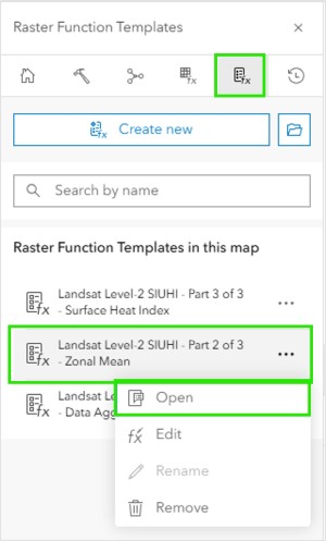
Step 1: Open the first RFT. Within the Analysis options , open the Raster Function Templates panel, click the three dots on Landsat Level-2 SIUHI – Part 2 of 3 – Zonal Mean, and select Open.

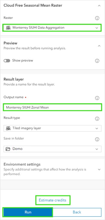
Step 2: With the input parameters panel now open, enter the required information and run the RFT. Select “Monterrey SIUHI Data Aggregation” as your input Raster, provide an output name of “Monterrey SIUHI Zonal Mean“, click Estimate credits and then Run.

Step 3: The result of Part 2 – Zonal Mean is a single band raster containing the mean surface temperature value of all vegetated pixels within the AOI . When processing completes, the resulting hosted imagery layer is saved to your organization and displayed in your map. Click Save to save your map. You are now ready for Analysis Part 3: Surface Heat Index.

Analysis Part 3: Surface Heat Index

The next part of the workflow is to calculate a surface heat index using the outputs from Part 1 and Part 2. This RFT uses the Extract Band, Band Arithmetic, Clip, and Zonal Statistics Raster Functions. The steps include:

• Calculate the difference between the seasonal mean surface temperature values from Part 1 and the vegetated mean value from Step 2.

The output is a per pixel index of surface temperature deviation from the vegetated mean surface temperature across the AOI. Relatively larger values indicative of more severe heat island effect.

Step 1: Open the first RFT.

1. Within the Analysis options, open the Raster Function Templates panel.
2. Click the three dots on Landsat Level-2 SIUHI – Part 3 of 3 – Surface Heat Index.
3. Select Open.

Step 2: With the input parameters panel now open, enter the required information and run the RFT.

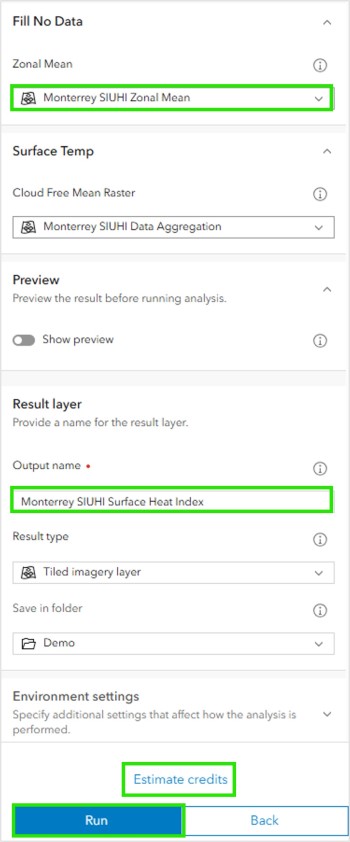
1. Select “Monterrey SIUHI Zonal Mean” as your input Zonal Mean Raster.
2. Select “Monterrey SUIHI Data Aggregation” as your Cloud Free Mean Raster.
3. Provide an output name of “Monterrey SIUHI Surface Heat Index“.
4. Click Estimate credits.
5. Click Run.

Step 3: The output of Part 3 – Surface Heat Index is a single band raster with a per pixel surface temperature deviation from the vegetated mean surface temperature across the AOI. Larger values indicate more severe the heat island effect. When processing completes, the resulting hosted imagery layer is saved to your organization and displayed in your map. Click Save to save your map. You are now ready to assess the results.

Assess the results

By default, the Surface Heat Index layer displays as grey scale. To help visualize the layer, and distinguish surface heat severity across the AOI, you can apply a stretch with a color ramp.

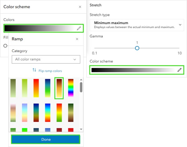
Step 1:  Go to the Styles tab and select Stretch Style Options.

Step 2:  Select a color ramp.

1. Within the Style options, click on Color scheme.
2. Click Colors to see a list of available color ramps.
3. In this case choose ‘Yellow to Dark Red‘.
4. Click Done.

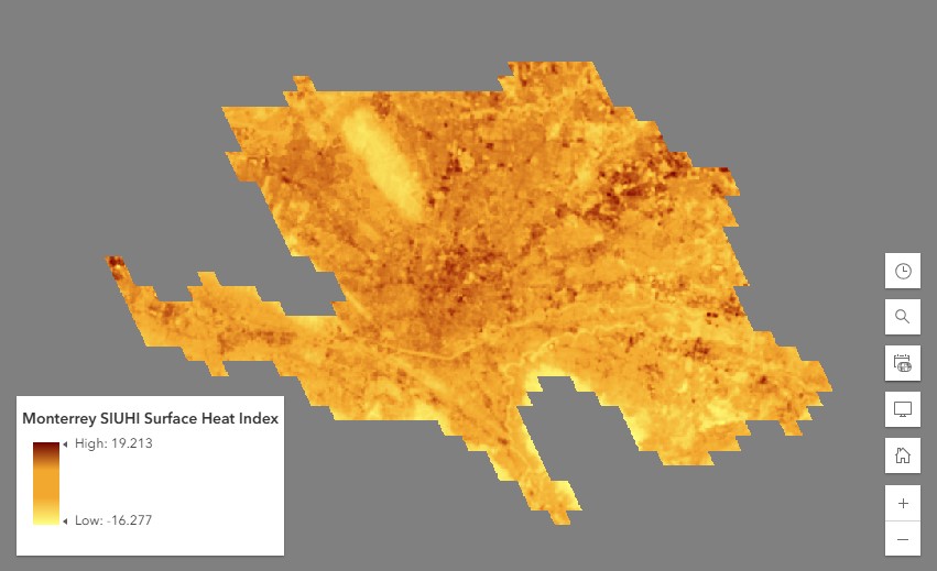
Step 3: Your output is now colorized. With the chosen color ramp, dark red represents the highest surface heat severity within the AOI.

This output layer can shared with your organization or publicly. It can be used in web applications for further analysis such as impact assessments and heat mitigation planning.

Some next steps for additional analysis could include one or more of the following:

• Running this workflow over time to show year over year heat trends for your area(s) of interest.
• Remap the output Surface Heat Index layer to heat severity classes, Convert Raster to Feature, and then enrich that feature layer with information such as population data using Zonal Statistics.
• Remap the output Surface Heat Index layer to heat severity classes and use that classified raster to enrich local census tracts with Zonal Statistics.

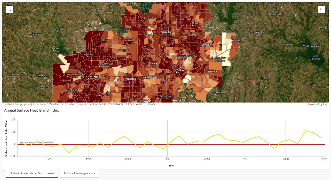
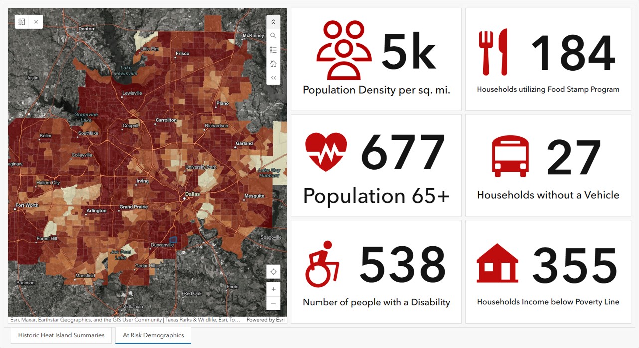
The following example dashboard was created combining a couple of the examples from above. We looked at Dallas, TX and created annual urban heat maps from 1985 to present to analyze trends over time by census tract. We also analyzed how heat severity is impacting different demographics across census tracts.

Temporal Surface Heat Island Dashboard – enriched for Dallas, Texas

Historic tab

At Risk  tab

Look for a follow up blog tutorial to describe how we created this dashboard.