Over the past year since the beta version of the Global Hexagons for Biodiversity and Conservation was released, we’ve heard amazing stories of the GIS community leveraging this resource to report on conservation targets and plan for the future. For example, a common workflow would include filtering areas for high biodiversity or threatened species, then excluding those hexagons if they’re currently protected, and then looking at the types of ecosystems or land use characteristics of the remaining hexagons to align with 30×30 goals.
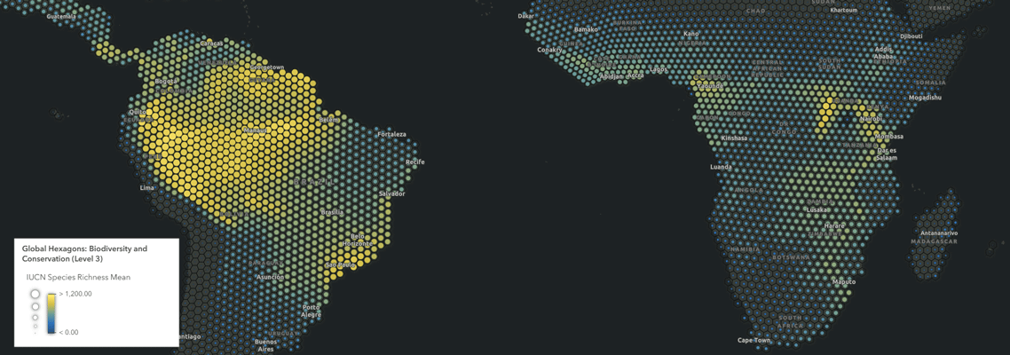
Using the Global Hexagons for Biodiversity and Conservation means that this work can be done in minutes rather than days. We are continuing to support this process and now have an improved version of the Global Hexagons for Biodiversity and Conservation.
What has changed?
- Updated data, where available. Also, the ESA WorldCover land cover product was removed since the data was not being updated by the source. All land cover is based on the Esri Sentinel-2 10m Land Use Land Cover product.
- All units have been harmonized across datasets and statistics. For example, all linear and aerial units are in meters rather than a mix of kilometers and meters. Bivariate or composite index maps that combine aerial measures are now more easily comparable.
- Implemented a new methodology for spatially summarizing partial pixel data that falls within a hexagon, which should result in capturing more extreme values in the minimum and maximum statistics. Applying a weighted value of that partial pixel also improves the accuracy of mean and predominant statistics.
- Additional statistics for some datasets, including precalculated percentages. There are now 82 summary statistics.
- More meaningful field aliases and long field descriptions.
- Data architecture that relies on 1 layer with sublayers rather than a group layer.
Using the Global Hexagons for Biodiversity and Conservation
Besides the workflow mentioned above, there are so many ways to analyze or visualize the data within the Hexagons, such as
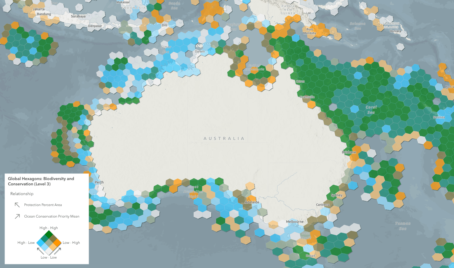
- Create multivariate maps
- Use one variable to filter or apply feature-specific effects to emphasize another
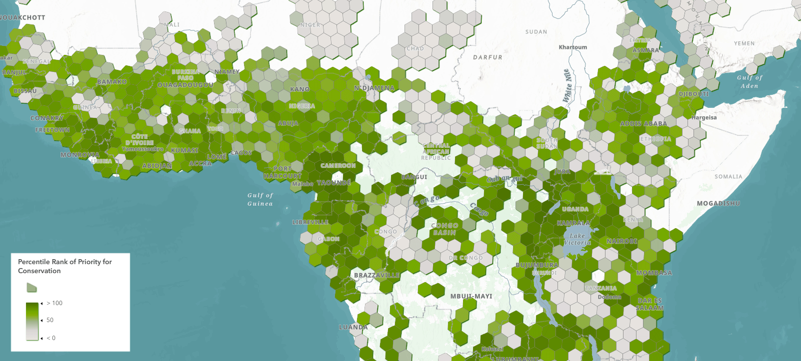
- Calculate a Composite Index of multiple variables
- Use the Find Similar tool
- Summarize your own data using blank H3 hexagons and join the fields using the GRID ID/Hexagon ID.

Article Discussion: