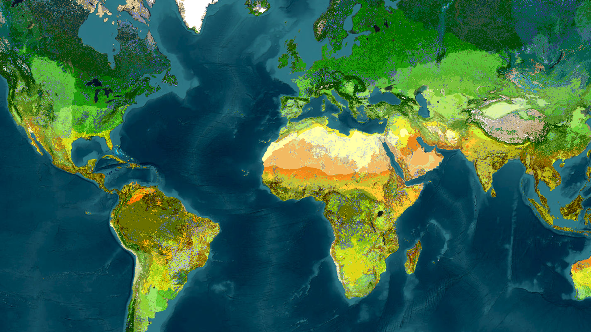
Web imagery layers can contain an enormous amount of information. The challenge is often not displaying the pixels—it is finding a clear way to explore their spatial patterns, compare categories, and connect chart observations back to image pixels on the map. Imagery charts provide that bridge.
In this blog, it walks through two examples. The first uses the World Terrestrial Ecosystems layer to explore ecosystem classes across the globe and within different regions. The second uses the Sentinel-2 Level-2A image collection to investigate spectral patterns in the Amazon coastal flood zone. Together, they show how web imagery charts can support both thematic exploration and pixel-level identification.
Explore global ecosystem patterns with a bar chart
The World Terrestrial Ecosystems layer in ArcGIS Living Atlas of the World contains 431 classes. A map communicates where those classes occur, while a chart adds another perspective: it helps reveal which classes are most prevalent and how the distribution changes from one region to another.
In Map Viewer, open the Charts pane (right white toolbar) for the imagery layer and choose Bar chart. The available chart types also include Histogram and Scatterplot. They varies depending on the imagery layer properties.
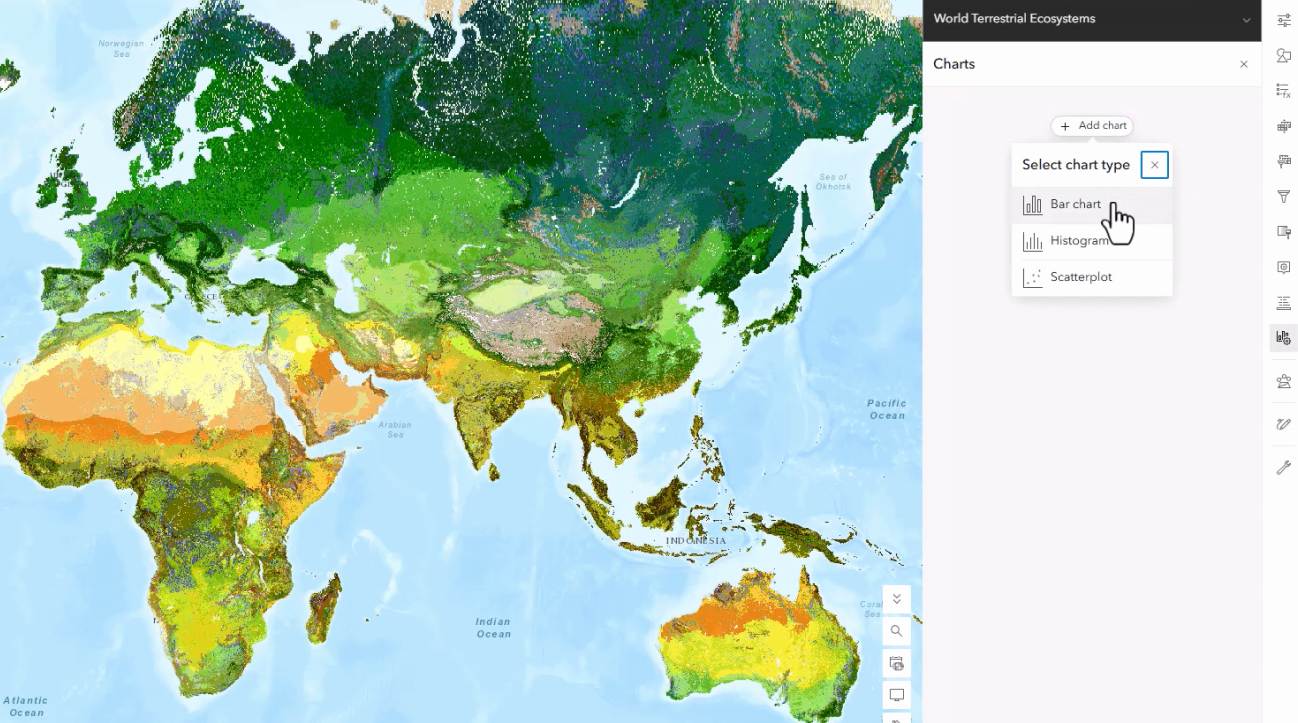
Configure categories, fields and groups
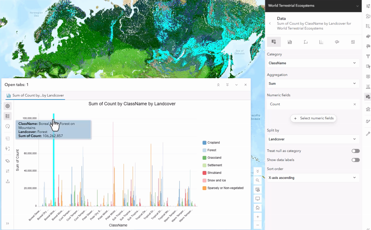
For this example, set field ClassName as the category, use Count as the numeric field with a Sum aggregation and split the results by Landcover. The resulting grouped bar chart summarizes the imagery by ecosystem classes while preserving the land-cover breakdown.
What the chart reveals
At the global extent, the largest class is the Boreal Mist Forest on Mountains. Selecting a bar highlights the corresponding pixels and see where the class occurs.
Let map extent become an analytical filter
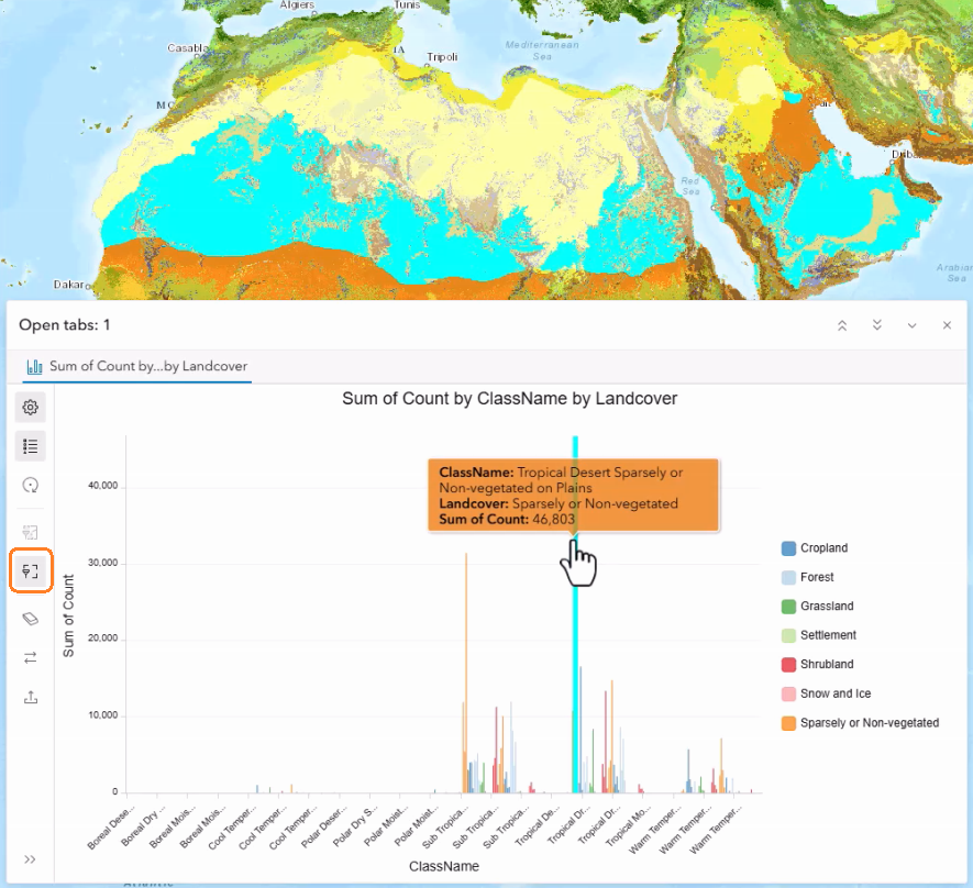
Global summaries are useful, but regional patterns can be very different. Turn on “Filter by extent” button in the chart to recalculate the chart for the current map view extent. As the map moves, the chart becomes a dynamic summary of the visible area. Tropical Desert on Plains is the largest class in Africa, while Tropical Moist Forest on Plains is dominant in South America. This extent-aware interaction makes it easy to compare regions without creating a separate analysis for each class.
Save the configured chart
Once the chart is configured, save the chart properties with the layer as a new layer item. The saved layer with the configured chart can become the source in the map, allowing the chart configuration to be reused in a later session or shared with others.
Use scatterplot on a large Sentinel-2 image collection
Imagery charts also work with large image collections. In the second workflow, we add the Sentinel-2 Level-2A layer to Map Viewer and navigates to an Amazon coastal flood zone.
Select image scenes with Image Collection Explorer
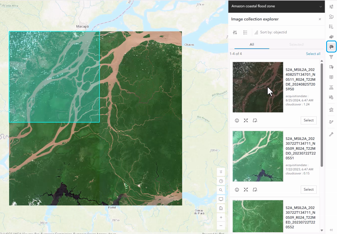
Open Image Collection Explorer to review the images available for the area of interest. The panel presents scene thumbnails and metadata, including image properties like acquisition dates and cloud-cover values. Here a small set of 4 Sentinel-2 scenes is selected and used to create a new layer focused on the study area.
Apply a short-wave infrared processing template
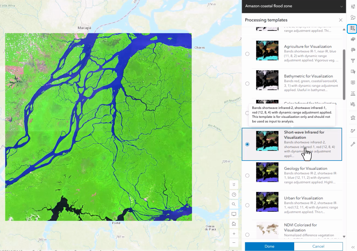
With the imagery layer selected, open Processing templates pane and switch to Short-wave Infrared for Visualization. In this rendering, water bodies become easier to distinguish from surrounding land, preparing the layer for further spectral exploration.
Identify spectral clusters with a scatterplot
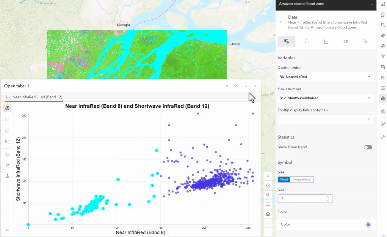
Create a scatterplot using Near InfraRed (Band 8) on the x-axis and Shortwave InfraRed (Band 12) on the y-axis. The chart plots pixel values from the imagery and exposes clusters that represent different spectral responses. Two clusters are clearly visible. Selecting a cluster in the chart highlights its pixels on the map, providing a fast way to identify the group associated with water bodies. The chart configuration also allows the axis variables to be changed to other available bands, such as Red (Band 4), supporting other similar spectral explorations.
From visual summary to spatial insight
These workflows demonstrate two typical uses of imagery charts. A bar chart can summarize a classified imagery layer and compare categories. A scatterplot can expose spectral structure and connect clusters to real locations. Whether you are studying global ecosystems or examining satellite scenes, imagery charts make complex raster information more approachable. They invite exploration, keep the map and chart synchronized, and help uncover valuable insights without leaving Map Viewer.
Web imagery charts support both tiled imagery layers and dynamic imagery layers, as well as the WCS imagery layers. We welcome you to explore those chart types and share your feedback with us.

Article Discussion: