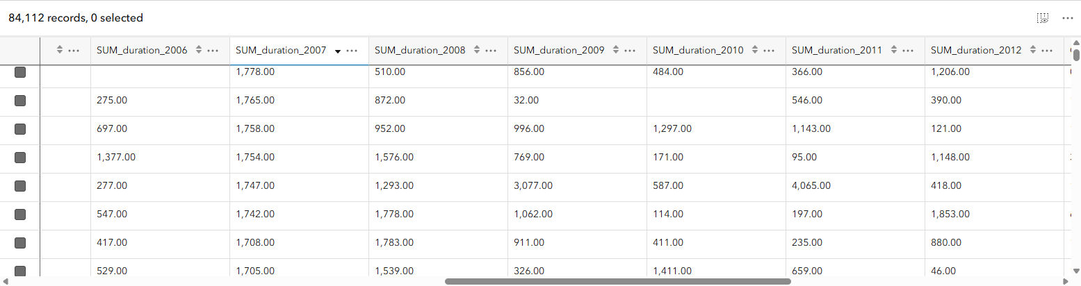
Time-series data represents how something changes over time. One way to store this information is in a wide table, where each feature appears only once and each time period is stored in a separate column.
For this blog, we’ll look at the amount of time census tracts spent under tornado warnings. Rather than creating a new census tract feature for every year, a single tract contains fields for 2006, 2007, 2008, through 2015. The geometry is stored only once, while the yearly values record the total number of minutes the census tract was under a tornado warning.
This structure can be especially useful for mapping because you can compare and calculate across the time fields without duplicating the feature’s geometry for every observation.
Tornado warnings don’t occur uniformly from year to year. Some places may experience warnings consistently, while others may see activity concentrated in only a few years. When your data contains measurements for several time periods, looking at those values individually can make broader patterns difficult to recognize.
Previously, a time series could show the value for each individual time period in a feature’s symbol, pop-up, or label. With the November 2026 release of Map Viewer, new time-series calculation methods allow us to go further and uncover additional patterns in the data.
Add a time series
Each census tract contains a field for every year, with its value representing the total minutes the tract was under a tornado warning during that year. We could symbolize any one of those fields, but looking at a single year tells only part of the story.
With our layer already published using a wide-table structure, we can configure these fields as a time series in Map Viewer and then choose calculation methods that help us explore how tornado-warning activity changes from year to year.
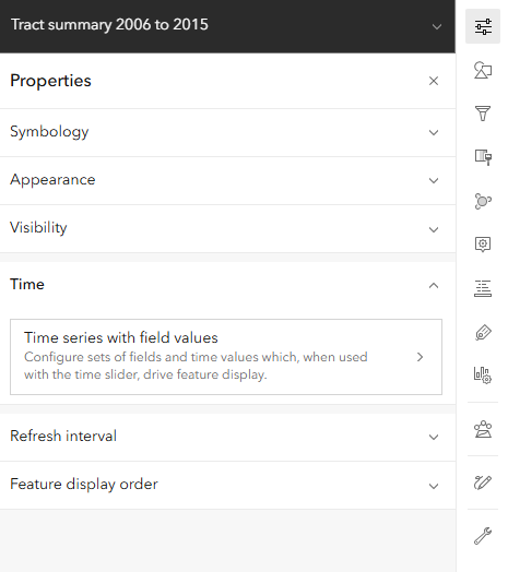
To get started, select the census tract layer and open the Properties panel. Find Time series, then click Add time series.
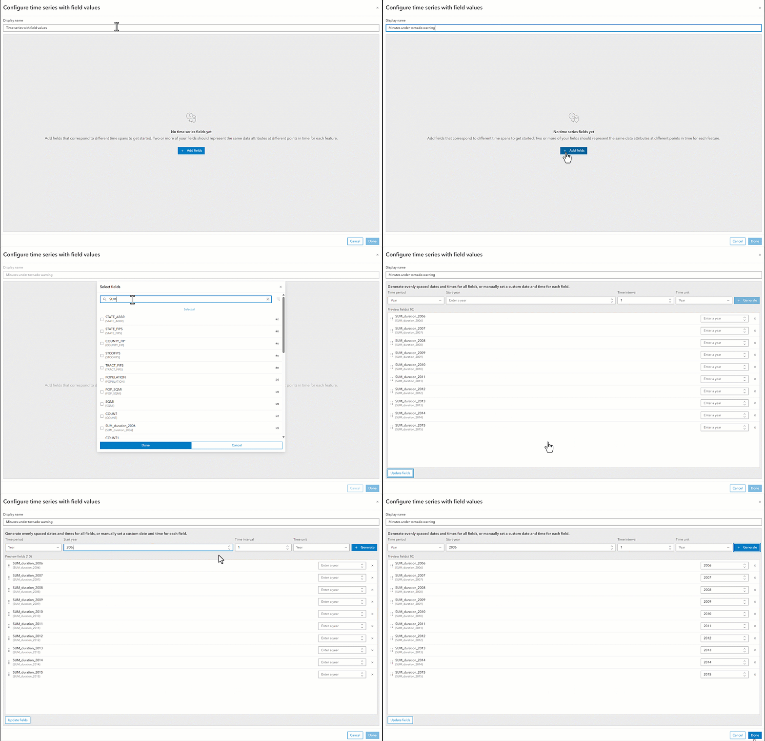
In the Configure time series dialog, give the time series a meaningful name. This is important because the name will be used when selecting the time series for styles, pop-ups, and labels, and it can also appear in the map legend.
Add the yearly fields
Next, we need to identify the fields that make up our time series.
Click Add field and select the fields containing the total tornado-warning minutes for each year. In our dataset, the series looks like this:
2006 → 2007 → 2008 → … → 2015
Each field represents one observation in the series, while the value stored in that field represents the total number of minutes the tract was under a tornado warning during that year.
Define the time period
Now we can define how those fields relate to time.
For this dataset, set the time period to Year. We know our first observation represents 2006, and each subsequent field advances the series by one year.
Once these properties are configured, click Generate. Map Viewer calculates a date for each field in the series. Those dates determine the positions of the observations on the time bar and allow Map Viewer to move through the fields chronologically.
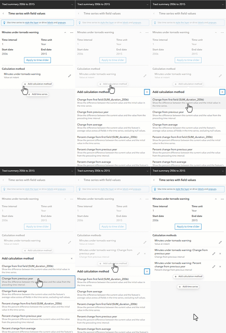
Add a calculation method
By default, the time series uses the value at an instant. This lets us move through the time series and see the value associated with each individual year.
But sometimes the value for a single year isn’t the pattern we’re interested in.
With the new calculation methods, we can derive additional information from the observations in the time series without creating new fields or doing additional preprocessing on the layer.
From the Time series panel, click Add calculation method and select a method from the available options. Multiple calculation methods can be configured as part of the same time series.
For this map, we’ll use percent change to answer a simple question:
How did the amount of time a census tract spent under tornado warnings change compared with the previous year?
Instead of simply mapping the number of minutes for each year, we can now map the percentage increase or decrease from the previous year.
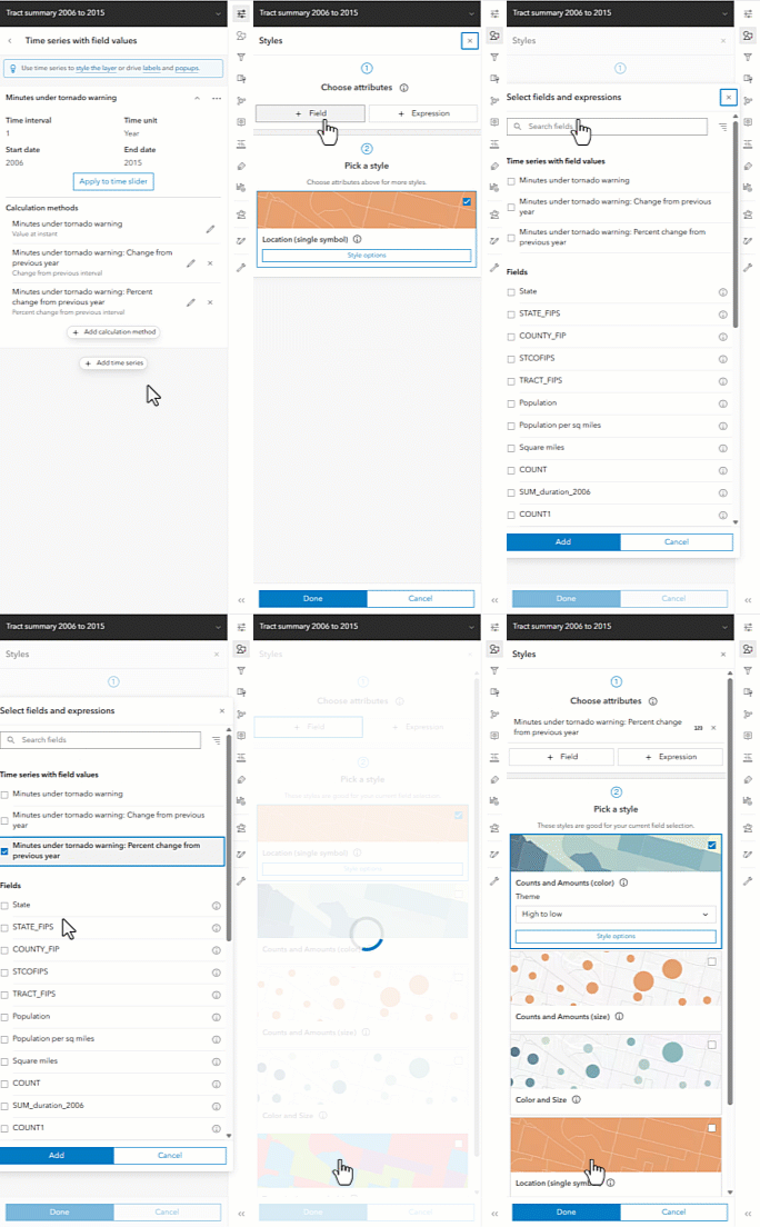
In the time series panel you will see a blue tooltip at the top. It has links that bring you to the panels in Map Viewer where you can use this time series. Clicking on styling which you will see in the gif below brings you to the Styles panel and in the field picker you see a category for all your time series that have been configured.
Style the calculated values
The Time series panel includes links to the places in Map Viewer where the configured time series can be used.
Select Styles to open the Styles panel. In the field picker, you’ll see a category containing the time series you configured, including its calculation methods.
For this example, we’ll select the percent change calculation and use the Counts and Amounts (color) style with the Above and Below theme.
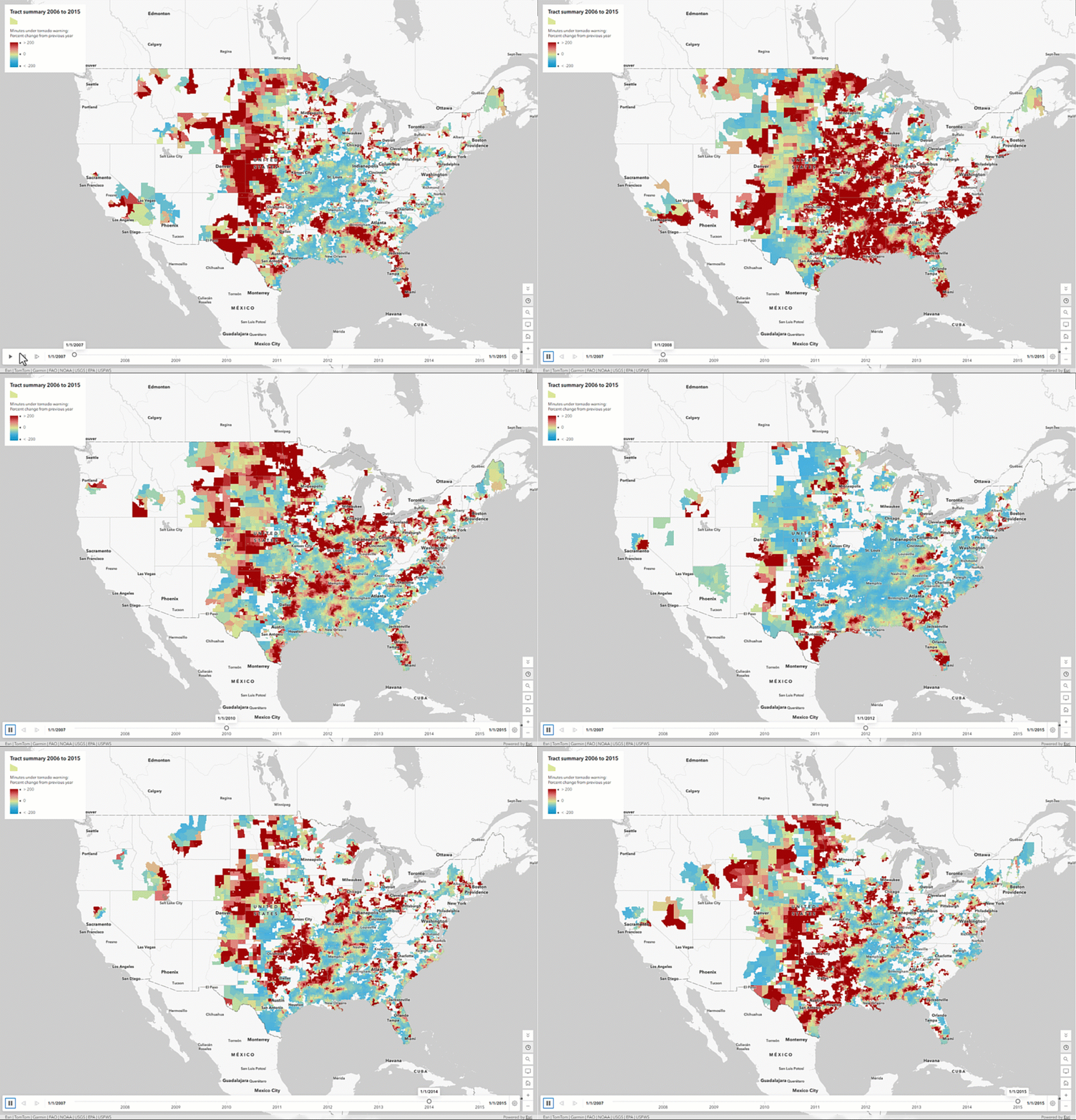
This gives the map an important new perspective. Instead of showing only which census tracts spent the most time under tornado warnings, we can see which tracts experienced an increase or decrease compared with the previous year.
Once the layer is styled using the time series, the time bar appears on the map. Play the animation to move through 2006–2015 and watch how the percent change in tornado-warning minutes varies geographically from year to year.
Use the time series throughout the map
Time-series calculations aren’t limited to styling.
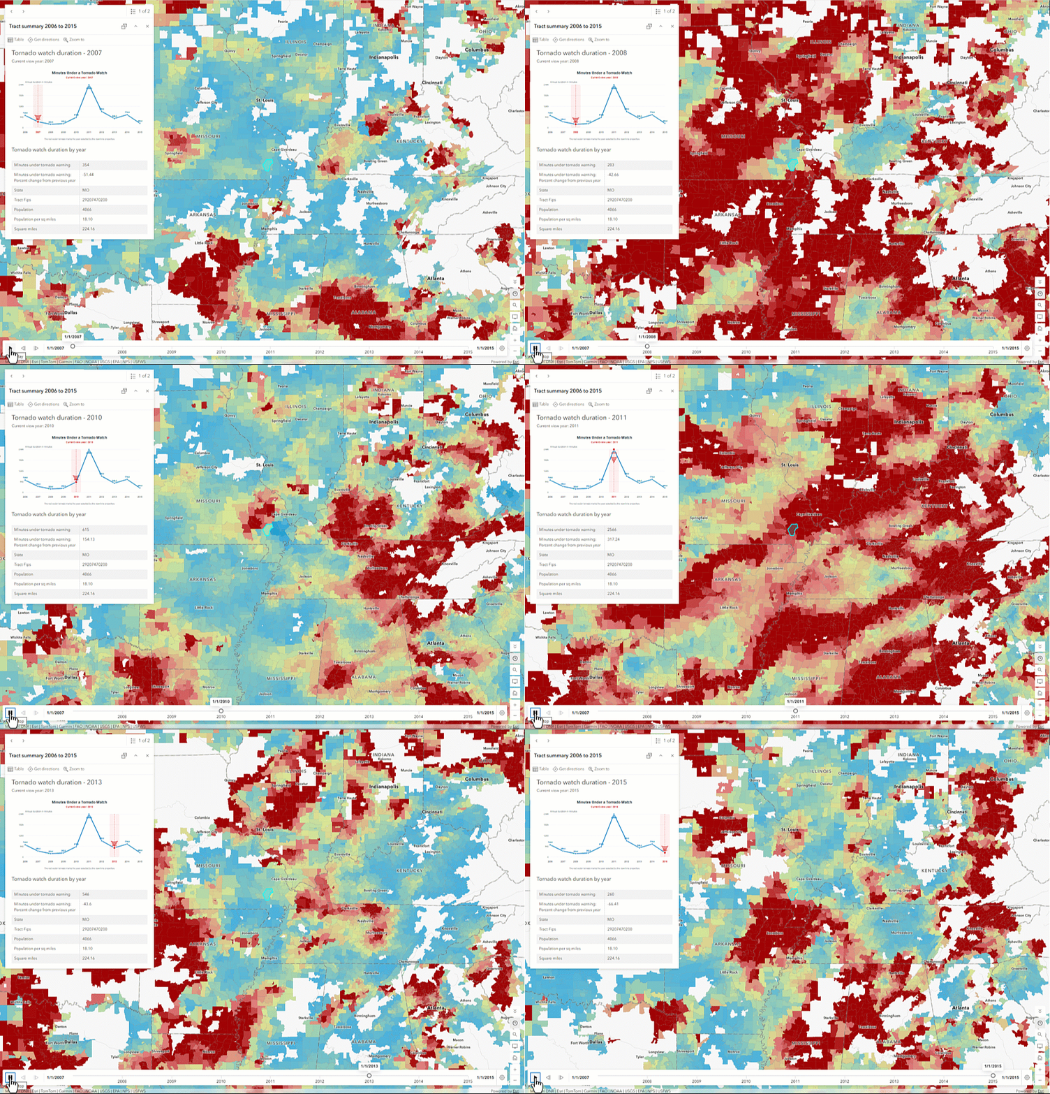
The same calculated values can also be used in pop-ups and labels. As the map progresses through time, the values displayed in the map’s symbols, labels, and pop-ups update with the current point in the series.
This allows the different parts of the map to tell the same temporal story. The symbology can reveal the overall geographic pattern, while labels and pop-ups provide the calculated values for individual census tracts.
Find the pattern behind the observations
A time series doesn’t have to be limited to showing one observation after another.
With calculation methods, we can use those observations to derive new information about how a feature is changing through time. In our tornado-warning example, the original fields tell us how many minutes each census tract was under a warning each year. Percent change transforms those individual observations into a measure of how warning activity is changing from one year to the next.
These calculation methods aren’t just another way to create a value. They let us transform a collection of observations into a characteristic we can map, animate, label, and explore.

Article Discussion: