You may not be surprised to learn that transportation in the United States is dominated by automobiles. Of all the miles traveled by American passengers in 2016, 86% occurred in cars (BTS 2017).

But did you know that fatal automobile accidents are a growing problem?
In just 2016, there were 34,439 reported fatal crashes, an increase of 12% since 2014!
The rise in fatal accidents cannot be simply attributed to more vehicles on roads; fatality rates per miles traveled have also increased: 2016 rates are nine percent higher than in 2014. It’s an unfortunate statistic, but before the day ends, more than 100 people will have likely lost their lives in the nation’s roads (NHTSA, Fatality Analysis Reporting System 2017).
How Can We Help Address the Problem?
Addressing this problem is an important but monumental task. There are millions of car accidents each year and limited available resources for the design and implementation of safety measures across the nation.
For this reason, finding and prioritizing locations where systemic issues result in multiple fatal car accidents is a crucial need for transportation agencies that run operations and guide safety policy. A spatial approach can help us expand beyond our basic understanding of where fatal car accidents occur and start detecting patterns that find these needles in the haystack.
Consider the following map, where nearly 35,000 fatal car accidents in the United States in 2016 have been distilled down to 60 specific locations to focus on based on the density of clusters of fatal crashes:
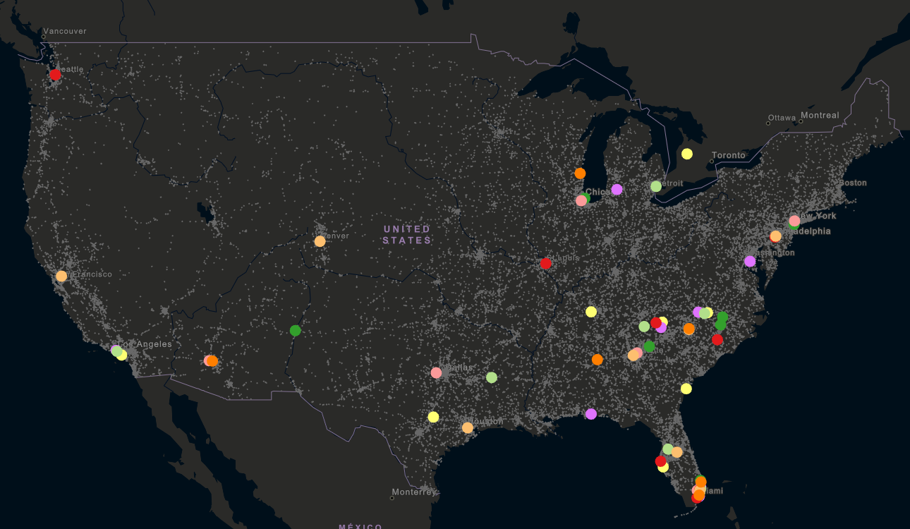
When applied, this type of spatial analysis can help us find the answer to the following question:
“Where are the locations that transportation agencies can focus on over the next year to ensure safety measures have the greatest impact?”
Methodology
Many fatal car accidents result from seemingly random events, but a dense cluster of fatal car accidents near a specific road segment can suggest the presence of a systemic problem or human-driven process that can greatly benefit from targeted safety measures. This methodology uses ArcGIS and a Spatial Statistics tool named Density-Based Clustering to find dense clusters of fatal car accidents. The clusters are our first “needles in the haystack”.
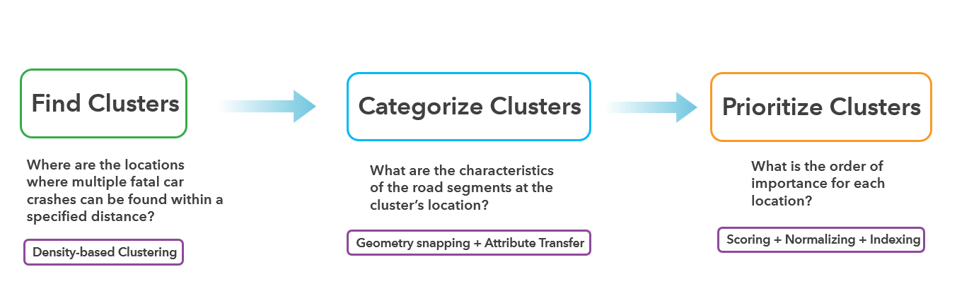
To organize and prioritize each cluster as a candidate safety measure project, we then consider the characteristics of each detected cluster and the transportation network:
- The elements of the transportation network at the cluster’s location, such as the presence of an intersection or the posted speed limit, become basis for classifying the clusters into groups that can be addressed by common safety measures. An example group would be “Intersection and Traffic Light Clusters”.
- The number of fatal accidents at the cluster and the traffic counts at the location then become the basis of prioritization rankings.
Let’s get started.
Establishing the Analysis Components
Before we begin finding clusters we need to answer a simple question:
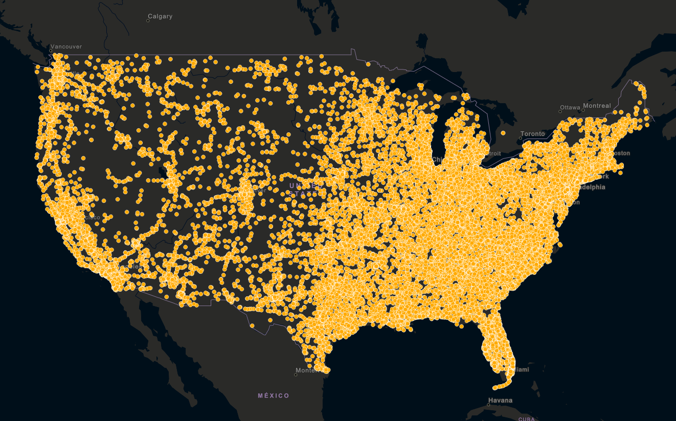
“Where are the fatal car accidents that occurred in the United States in 2016?”
The Fatality Analysis Reporting System (FARS) GIS data from the National Highway Traffic Safety Administration (NHTSA) serves as our starting point:
We will also use road data from the Federal Highway Administration (FHWA) Highway Performance Management System (HPMS) and All-Roads Network of Linear-Referenced Data (ARNOLD) database to provide us roadway characteristic information for each cluster.
With these ingredients we can start finding clusters!
Density-based Clustering
Let’s answer the following question:
“Where are the clusters of fatal car accidents with at least three separate incidents occurring within a 300-meter area?”
Since our data contains discrete fatal accidents across a full year, the answer to this question would be a useful first step to help us find road segments and intersections where a systemic safety problem may be at fault. With the Density-based Clustering tool applied to NHTSA’s Fatality Analysis Reporting System (FARS) data, finding this answer is a single step in ArcGIS.
What exactly is Density-based Clustering?
The Density-based Clustering tool works by detecting areas where observations are concentrated and where they are separated by areas that are empty or sparse. Observations that are not part of a cluster are labeled as noise.
The tool uses an unsupervised machine learning clustering algorithm named DBSCAN which automatically detects patterns based purely on spatial location and the distance to a specified number of neighbors. These algorithms are considered unsupervised because they do not require any training on what it means to be a cluster.
For this analysis, we want to start exploring with a specific definition of a cluster: we will provide a specified distance (300 meters) and minimum number of features per cluster (three accidents) to define and separate dense clusters from sparser noise.
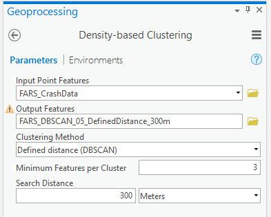
With these parameters specified, the output yields 60 clusters that satisfy our criteria:

Let’s explore a few of these clusters…
One cluster was found in Maryland at the intersection of State Route 5 and Earnshaw Drive/Burch Hill Road:
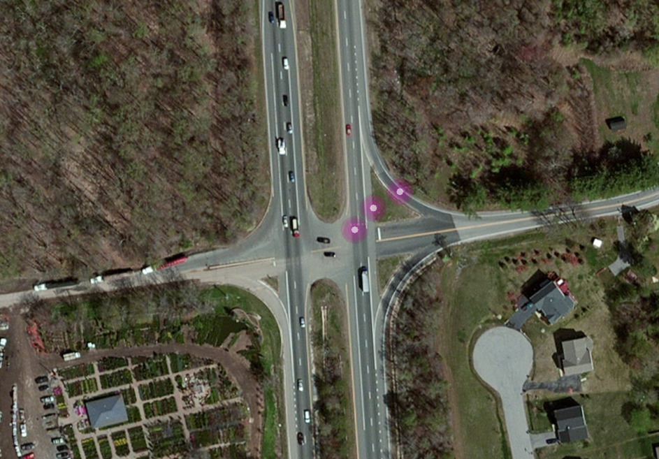
With three separate fatal car accidents in a single year at this intersection, it is possible that safety measures are needed to save lives. We can target this location for further investigation and explore further.
Does this intersection need a traffic light?
What are the speed limits at this intersection?
Are there objects that obstruct the visibility of incoming traffic at different angles in this intersection?
Let’s explore another cluster near Clayton, California:
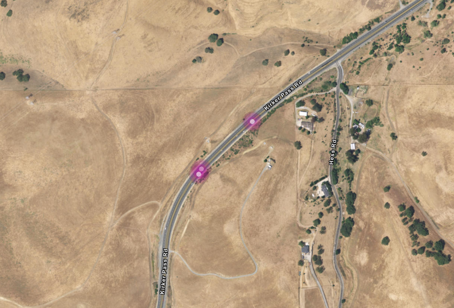
In this case, three high-speed fatal car accidents occurred near a curve of the Kirker Pass Rd. With this information, could we now work with domain experts to help investigate if speed limits or curve signage are needed to help drivers safely navigate this road?
Categorizing Clusters
Filtering thousands of fatal car accidents into 60 clusters has led us to additional interesting questions. To help mobilize with safety measures, we can use additional location data from the transportation network to classify and prioritize each cluster.
Cluster Coincident Road Segments
Let’s begin by further filtering the 60 clusters into clusters where all accidents occurred in the same road segment. The purpose of this step is to find the “sharpest needles in the haystack”, or the clusters where the incidents are all related to the same transportation network feature and are more likely to benefit from a single safety measure.
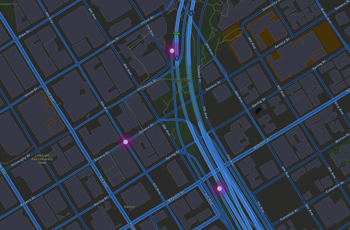
Consider the following cluster, where three accidents are in different roads:
And the following cluster, where all three accidents occurred in the same segment:
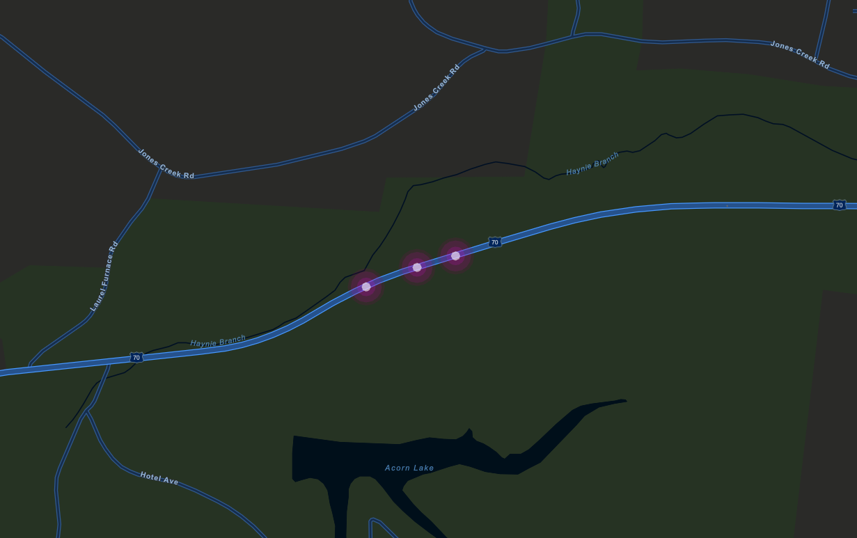
Which one would you prioritize as a transportation analyst?
A safety measure in this road segment is likely to be more impactful than a safety measure in one of the three road segments in the previous cluster. For this reason, the clusters with features in coincident road segments receive a higher priority in our analysis.
Cluster Attributes
We continue to add information to each cluster according to the characteristics of the road network near the incidents. A few examples are: the presence of an intersection, the type of intersection, the presence of a pedestrian crossing, the speed limit, the curvature, and others.
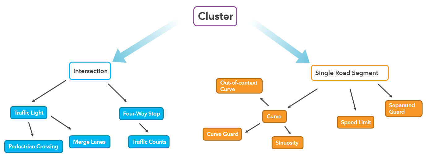
The goal is to start classifying each cluster so that safety measures that can help in one group can be considered for other, similar locations. Example groups include:
- “Intersection with Traffic Light”
- “Single Road Segment with Out-of-Context Curve”
- “Pedestrian-Heavy”
- “Highway Interchange”
Additionally, the outputs will be organized into these groups to help transportation agencies navigate around important locations based on the type of transportation network at each location.
Prioritizing Clusters
Once all clusters have been organized into discrete groups and contain roadway characteristic attributes, we can start determining the priority for each cluster.
To do this, we produce a “priority score” for each cluster, initially based on the number of fatal accidents and the amount of traffic at the road segment for the cluster.
Future refinements of this analysis would incorporate additional components for the priority score; for example: rates of increase of fatal accidents in the region, or demographic social vulnerability.
The priority score determines the priority rank for each cluster:
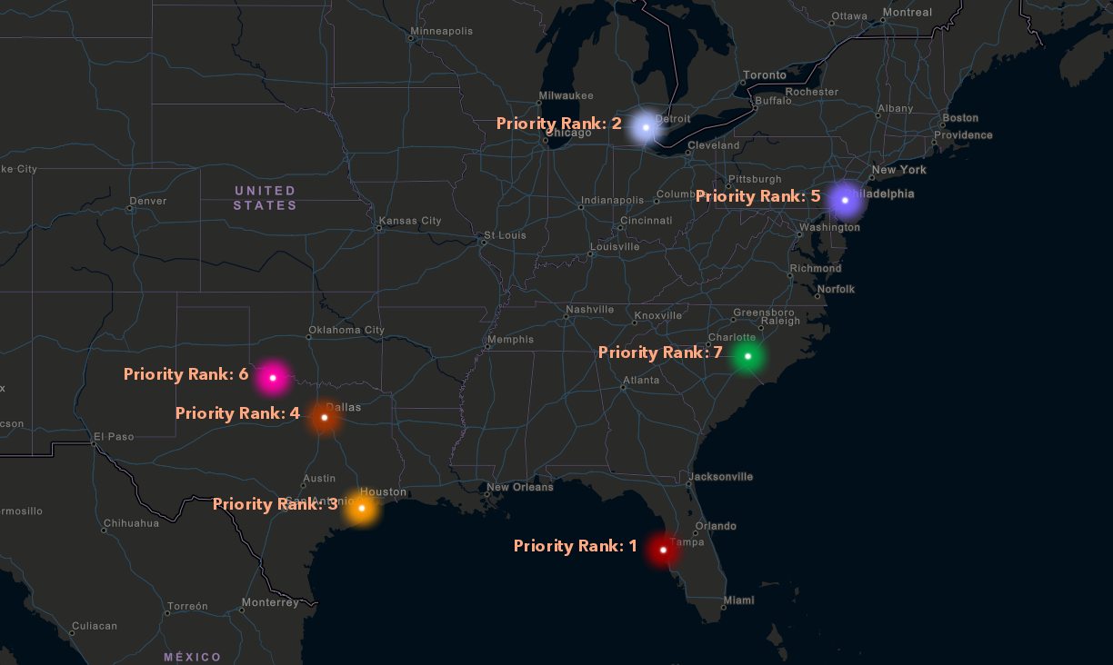
An initial pass finds these needles in the haystack but this is only the beginning.
Next Steps
Our next steps are to incorporate additional metrics, such as the previously mentioned cluster groups, for comparisons between clusters.
Once clusters receive further descriptive information, we can then prioritize ranks at three grouping levels:
- National
- State
- Cluster Group
National rankings correspond to ranked priority score comparisons for all clusters in the United States. A few states, such as Florida and North Carolina, have a higher number of clusters, so a state-wide rank is intended to assist state transportation agencies prioritize within their context.
Finally, the cluster groups from the hierarchy defined in the previous segment receive their own group rankings, with the intent to assist transportation agencies when organizing safety measure efforts among their groups with domain expertise for each type of traffic accident problem.
The output of this analysis is defined as the fatal car accident clusters with priority rankings at each level. Organized needles in a haystack.
Takeaways
With millions of vehicle accidents and thousands of fatal car crashes in the United States each year, finding and prioritizing locations where systemic issues result in multiple fatal car accidents is a crucial need for transportation agencies that run operations and guide safety policy. A spatial approach can help us expand beyond our basic understanding of where fatal car accidents occur and start detecting important patterns that find these needles in the haystack.
In our analysis, we identified these important locations using Density-based Clustering, an approach that identifies clusters based on the concentration of accidents in space. For this example, we used a simple definition of what a cluster means (300 meters; three accidents minimum per cluster), but the tool is also able to discern the meaning of a cluster from the provided data.
These clusters became our candidate priority locations, and we then supplement additional characteristics for each cluster to categorize and prioritize.
It is important to recognize that this is not the end of this analysis, and that Density-based Clustering is an important step in a series of steps to ask questions, explore the available data, perform analysis, and interpret our results. With Density-based Clustering, we can quickly start answering some of the most interesting exploratory questions and continue progressing in our understanding of this problem.
Resources
Examples:
Data:
References
BTS, USDOT. 2017. U.S. Vehicle-Miles. https://www.bts.gov/content/us-vehicle-miles-millions.
NHTSA, USDOT. 2017. Fatality Analysis Reporting System. https://www.nhtsa.gov/research-data/fatality-analysis-reporting-system-fars.
—. 2016. Transportation Quick Facts. https://crashstats.nhtsa.dot.gov/Api/Public/ViewPublication/812451.

Article Discussion: