We are fortunate to be living in an era where data is coming at us quickly. But are we using our temporal data to its full analytical potential? Animations, charts, and trend maps are useful visualizations that can help us start to understand our temporal data. These have their strengths, but also their weaknesses—an animation can be overwhelming and can’t be conveyed in print, and lots of valuable information is lost and oversimplified with charts and trend maps.
With ArcGIS Pro 2.5, you can now apply space-time statistics and visualizations to your raster time series data. The Space Time Pattern Mining toolbox contains statistical tools to analyze and map data distributions and patterns in both space and time. It was previously limited to vector (point and polygon) data. Opening up the capabilities of the Space Time Pattern Mining tools with the release of ArcGIS Pro 2.5 to raster data provides many new mapping and analytical opportunities. In this blog article, you will learn what types of analysis are possible with the Space Time Pattern Mining toolbox, and how to prepare your raster data before analysis.
What is possible with space time pattern mining?
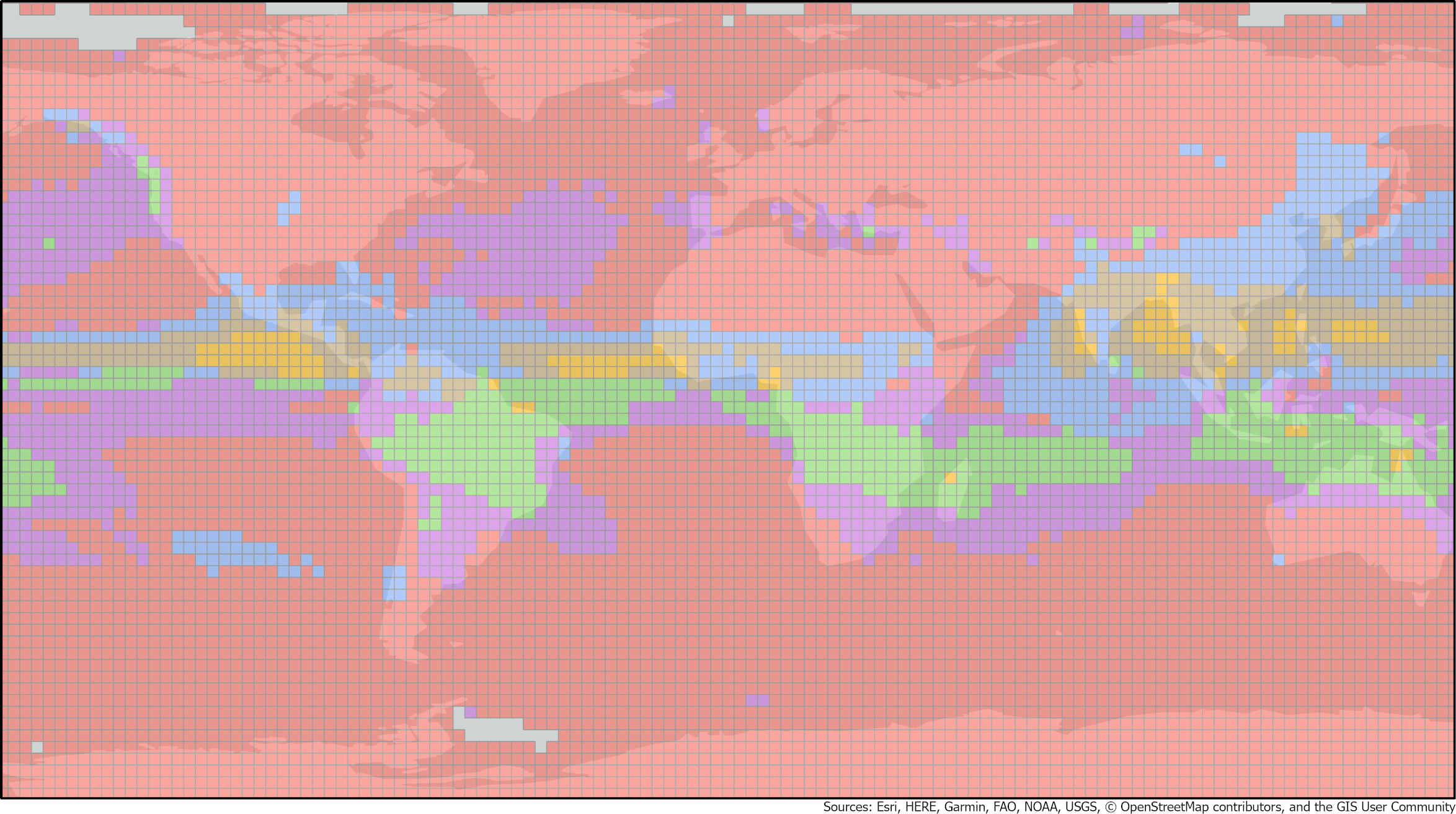
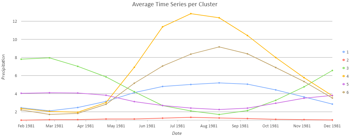
There are many analysis tools available in the Space Time Pattern Mining toolbox, including the Time Series Clustering tool. With the Time Series Clustering tool, you can identify areas where precipitation patterns are similar annually:
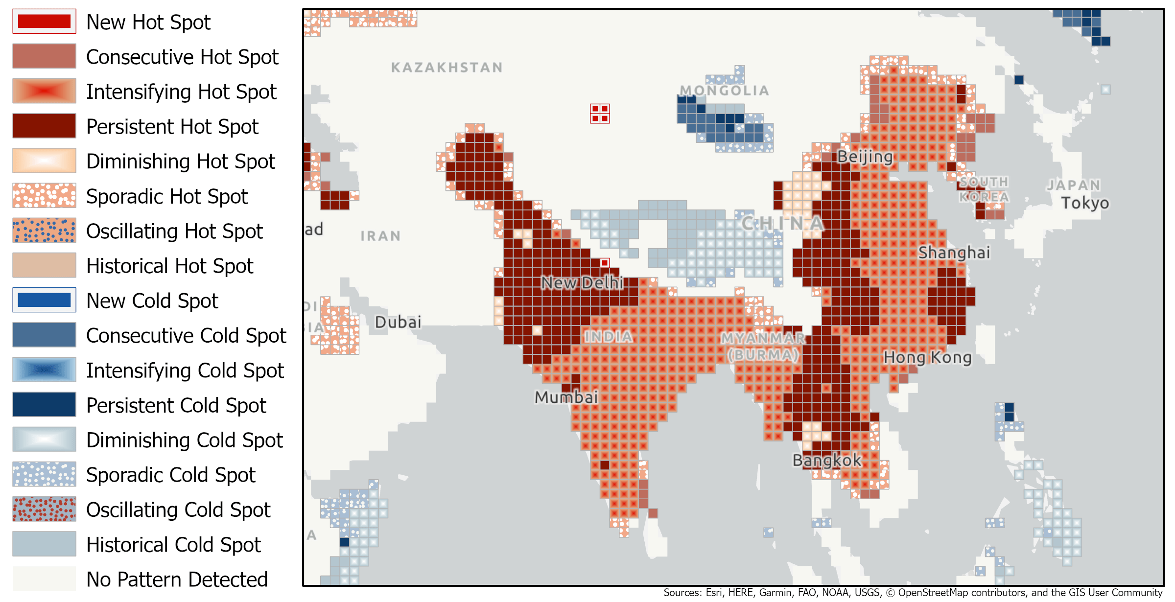
With the Emerging Hot Spot Analysis tool, you can find hot and cold spots of pollution—areas of high and low pollution values when compared to the overall study area. The output of the tool breaks down the results into 17 categories representing the temporal trends of hot and cold spots over time.
The Space Time Pattern Mining toolbox also contains the analysis tool Local Outlier Analysis, which can be used to find clusters and outliers in your analysis variables. Several space-time utility tools are also available with ArcGIS Pro, including tools that can be used to visualize the space-time cube data and analysis results in 2D and 3D. An add-in to help you with the visualization of the space-time cube data is also available at esriurl.com/SpaceTimeCubeExplorer.
How can I create a space-time cube from raster data?
The space-time cube is the fundamental data type for use in the Space Time Pattern Mining toolbox. You can create space-time cubes from point and polygon vector data, but this blog article will focus on how to create them from raster data. Some raster data formats require more processing than others before you can create a space-time cube. Instructions for three common data types are below:
Figure 4 summarizes the main workflow from each of these data types into a space-time cube.

Make a space-time cube with .tif data
To create a space-time cube with a temporal .tif file format, the steps of the workflow are: loading the .tif files into a mosaic, creating a multidimensional raster layer, then creating a space-time cube. The workflow can be modified to use not just .tif files, but any valid raster input to a mosaic.
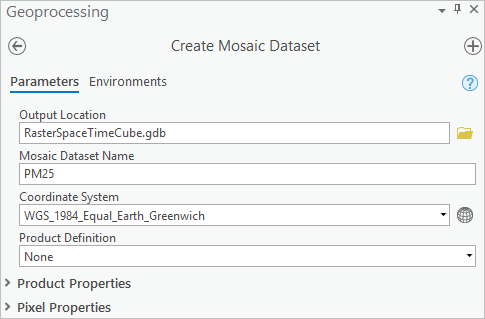
1. First, you’ll create an empty mosaic dataset using the Create Mosaic Dataset. To create the mosaic, fill in the following parameters:
- Output Location: any geodatabase of your choice.
- Mosaic Dataset Name: PM25 (or an appropriate name if you are using your own data).
- Coordinate System: The coordinate system of the current map will be available in the drop-down menu. Choose Equal Earth (world) in the Coordinate System window if you want to match the coordinate system of the downloaded pollution data.
- Product Definition: None.
2. Next, you’ll add rasters to the empty mosaic dataset using the Add Rasters to Mosaic Dataset tool with the following parameters:
- Mosaic Dataset: PM25 (or the name you used in step 1)
- Raster Type: Raster Dataset
- Processing Templates: Default
- Input Data: Folder
- Click the Browse button under the Input Data parameter, browse to the folder that contains your raster data folder, then click OK.

3. Create and populate a Variable field in the mosaic Footprints table using the Calculate Field The mosaic has three parts—the Boundary, Footprint, and Image. The Footprint is a layer representing the footprint of each raster, with attributes for each raster in the table. Use the following parameters in the Calculate Field tool:
- Input Table: PM25\Footprint (or the footprint table from another mosaic if you are using your own data)
- Field Name (Existing or New): Variable
- Field Type: Text
- Expression Type: Python 3
- Variable = : “PM 2.5” (or an appropriate variable name if you are using your own data)

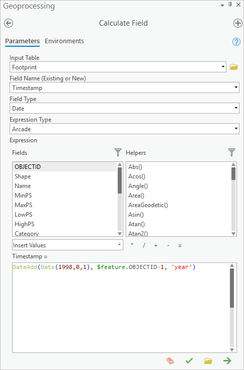
4. Create and populate a Timestamp field in the mosaic Footprints table using the Calculate Field You can use an Arcade expression to increment the date of each footprint by a year, starting from 1998. Use the following parameters in the tool:
- Input Table: PM25\Footprint (or the footprint table from another mosaic if you are using your own data)
- Field Name (Existing or New): Timestamp
- Field Type: Date
- Expression Type: Arcade
- Timestamp = : DateAdd(Date(1998,0,1), $feature.OBJECTID-1, ‘year’) (or an appropriate expression if you are using your own data)
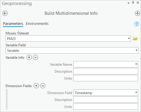
5. Time enable the mosaic using the Build Multidimensional Info This tool converts the Variable and Timestamp fields into the correct format, so that ArcGIS Pro can recognize the temporal data. Use the following parameters in the tool:
- Mosaic Dataset: PM25 (or the name you used in step 1)
- Variable Field: Variable
- Dimension Field: Timestamp
6. Since time in ArcGIS Pro can act as a filter, turn off time on the mosaic by right-clicking the mosaic, then changing Layer Time to No Time in the Time tab. This step is best practice to avoid unexpected time ranges in your results.
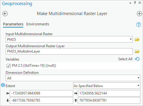
7. Convert the time-enabled mosaic into a single time-enabled layer compatible with many tools in ArcGIS Pro using the Make Multidimensional Raster Layer tool with the following parameters:
- Input Multidimensional Raster Layer: PM25
- All other parameters will autopopulate
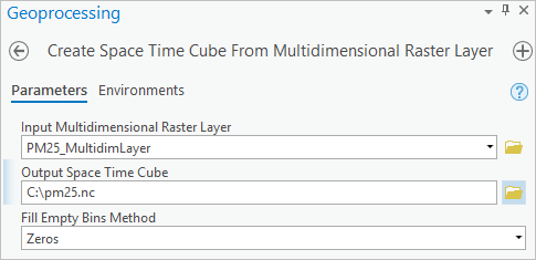
8. Then, you’ll use the Create Space Time Cube from Multidimensional Raster Layer tool to create a space-time cube. If you happen to have empty bins in the newly created cube, this tool allows you to choose from several methods to fill them. This is important because you need to have a complete time series for each location in the cube to perform analysis of the cube. Configure the tool using the following parameters:
- Input Multidimensional Raster Layer: PM25_MultidimLayer
- Output Space Time Cube: any path you’d like to save the space-time cube
- Fill Empty Bins Method: Zeros
9. You now have a space-time cube that is ready for space time pattern mining analysis. Try using your new space-time cube with one of the tools from the beginning of this blog article: Time Series Clustering, Emerging Hot Spot Analysis, or Local Outlier Analysis. If you’ve been following along using the PM 2.5 space-time cube, you can configure the Emerging Hot Spot Analysis tool as follows:
- Input Space Time Cube: the path you chose in step 8 to save your space-time cube
- Analysis Variable: PM 2.5_NONE_ZEROS
- Output Features: pm25_EmergingHotSpotAnalysis
- Conceptualization of Spatial Relationships: K nearest neighbors
- Number of Spatial Neighbors: 8
- Neighborhood Time Step: 1
- Define Global Window: Individual time step
The results of the Emerging Hot Spot Analysis tool with the PM 2.5 space-time cube were featured in Figure 3—if you’ve followed the workflow using this data, your results should match.
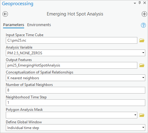
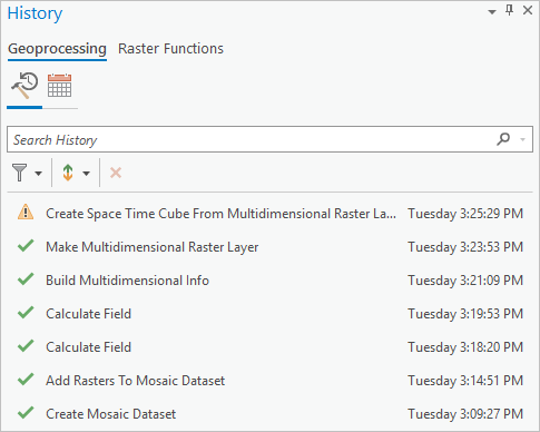
Figure 13 shows the full workflow from the beginning .tif files (step 1) to the newly created space-time cube (step 8) as items in the History pane (from the first tool at the bottom, to the last tool at the top).
Make a space-time cube with netCDF data
A netCDF file is a scientific data format that many organizations use to publish multidimensional data. The space-time cube is a specially configured netCDF file for use with the tools in the Space Time Pattern Mining toolbox. However, you can load any netCDF file into a space-time cube using a short workflow that repeats some of the steps from the above workflow using .tif files:
1. The first step is to create a multidimensional raster layer, which can be done in two ways. Either use the Make Multidimensional Raster Layer tool (as shown in step 5 above) or through the Add Data drop-down menu on the Map ribbon (choose Multidimensional Raster Layer).
2. Then, as before, create a netCDF space-time cube from the multidimensional raster layer using the Create Space Time Cube from Multidimensional Raster Layer
Make a space-time cube with .crf data
Creating a space-time cube using a .crf file is the most straightforward way to create space-time cubes from multidimensional raster layers. These can be loaded straight into a space-time cube. The workflow of creating space-time cubes using .crf files is as follows:
1. As shown above, use the Create Space Time Cube from Multidimensional Raster Layer tool to create a netCDF space-time cube from the multidimensional raster layer. If your .crf file has multiple variables, the Create Space Time Cube from Multidimensional Raster Layer tool will create the space-time cube using the first temporal variable. If you want to use another variable, you should first use the Make Multidimensional Raster Layer tool, which will allow you to select which variable to use.
How can I optimize my space-time cube?

Limit the spatial extent
Space-time cubes can get very large very quickly, especially when derived from multidimensional raster data. This may make the analysis of your space-time cube slow to compute or slow to render and visualize. On the Environments tab of the Create Space Time Cube from Multidimensional Raster Layer tool, Extent can be used to limit the spatial extent used for the space-time cube. This can be useful, for example, if you have a netCDF file with global data, but you want to perform your analysis in a single country. You can use the Extent parameter to limit the space-time cube extent by geometry, display extent, or other methods.
Limit the temporal extent
Likewise, another way of limiting the size of your space-time cube, and improving performance, is to limit the temporal extent. For example, you may have climate data for 100 years, but are only interested in analyzing the last 30 years. To restrict your space-time cube to 30 years, you can filter the multidimensional raster layer you use as input to the Create Space Time Cube from Multidimensional Raster Layer tool. This can be done by using the Dimension Definition in either the Make Multidimensional Raster Layer tool or the Subset Multidimensional Raster tool.
Best practices when creating your space-time cube from rasters
It is important to apply spatial and temporal filtering to the space and time that you are interested in, even if computation is not an issue. Restricting the spatial extent is important because many of the analysis tools, for example, Local Outlier Analysis, will compare a local neighborhood to the global data to calculate statistics. If your global data includes locations you are not interested in, the results may not be applicable to the question you are trying to answer. Similarly, your results will be adversely impacted if you use a temporal extent greater than the time period in which you are interested. For example, the Emerging Hot Spot Analysis tool finds many types of hot and cold spot patterns over time, including newly developed hot and cold spots. The new hot and cold spots are dependent on the behavior of the location throughout the time series and, most importantly, what is happening in the last time step. If the last time step is later than the time window you are interested in, you may not find new hot and cold spots that reflect the question you are trying to answer.
Resampling
Another method of improving the analysis performance of your space-time cube created from raster data is by resampling. The space-time cube will have one space-time bin per raster cell. If your raster cell resolution is higher than the space-time cube bin size that you need, you can use the Resample tool (or any other tool that will resample, for example, Project Raster) before creating the space-time cube to make the resolution coarser. Remember that resampling data can have a smoothing effect on the values in the dataset, therefore there may be patterns that are apparent at one resolution, but not at another. It is important when deciding the scale of your analysis to ask yourself whether there is a spatial resolution that is most appropriate for the question you are trying to answer.
Further resources
You can follow this Learn lesson to walk through a guided analysis workflow, which includes creating the pollution hot spot example depicted in Figure 3 above.
The Spatial Statistics team at Esri has curated many resources at http://esriurl.com/spatialstats including the following:
- The Space Time Cube Explorer Add-In to help visualize your space-time cube in both 2D and 3D
- A case study using Space Time Pattern Mining to analyze violent crime
- A learn lesson that uses rasters and machine learning to downscale climate data
Happy analyzing!
P.S. The Spatial Statistics team is continually working on new tools and capabilities to help you in your analysis workflow—we think you will be really excited about the newest Space Time Pattern Mining capabilities coming soon!
References
PM 2.5 pollution data:
- van Donkelaar, A., R. V. Martin, M. Brauer, N. C. Hsu, R. A. Kahn, R. C. Levy, A. Lyapustin, A. M. Sayer, and D. M. Winker. 2018. Global Annual PM2.5 Grids from MODIS, MISR and SeaWiFS Aerosol Optical Depth (AOD) with GWR, 1998-2016. Palisades, NY: NASA Socioeconomic Data and Applications Center (SEDAC). https://doi.org/10.7927/H4ZK5DQS. Accessed 27 Jan 2020.
- van Donkelaar, A., R. V. Martin, M. Brauer, N. C. Hsu, R. A. Kahn, R. C. Levy, A. Lyapustin, A. M. Sayer, and D. M. Winker. 2016. Global Estimates of Fine Particulate Matter Using a Combined Geophysical-Statistical Method with Information from Satellites. Environmental Science & Technology 50 (7): 3762-3772. https://doi.org/10.1021/acs.est.5b05833.
Global precipitation data:
- CMAP precipitation data provided by the NOAA/OAR/ESRL PSD, Boulder, Colorado, USA, from their Website at https://www.esrl.noaa.gov/psd/
- Xie, P., and P.A. Arkin, 1997: Global precipitation: A 17-year monthly analysis based on gauge observations, satellite estimates, and numerical model outputs. Bull. Amer. Meteor. Soc., 78, 2539 – 2558.

Commenting is not enabled for this article.