When searching for a new home, we all weigh different features: “I’d pay $10,000 more for an extra bedroom,” or “Let’s reduce by $5,000 because there’s no basement.” Each of these value judgments adds up to the total price you’re willing to pay. We are introducing new functionality in ArcGIS Pro that can break down your predictions in the same way.
With ArcGIS Pro 3.8, we have introduced a powerful new feature in the Evaluate Variable Influence for Predictions tool: SHAP values. This enhancement brings transparency to your predictive models by showing exactly how each input variable contributes to every prediction.
What Are SHAP Values?
SHAP (SHapley Additive exPlanations) values provide a detailed breakdown of model predictions, assigning a contribution value to each input variable. For example, if you’re predicting home prices, a SHAP breakdown might look like this:
Median Home Value (Intercept) = $300,000
4 bedrooms +$20,000
2 bathrooms +$5,000
2,000 sq. ft. +$2,000
Location -$15,000
Built in 1990 -$1,000
0.5 acre lot +$10,000
Total Predicted Value = $321,000
This breakdown shows how each variable nudges the prediction up or down, making your models more interpretable and actionable. These SHAP values then sum up to the predicted value and are in the units of the prediction, in this case U.S. Dollars.
Step-by-Step analysis with King County Housing Data
Let’s walk through a real-world example using housing data from King County, Washington:
for more information on this dataset and modeling questions, check out these prediction tutorials.
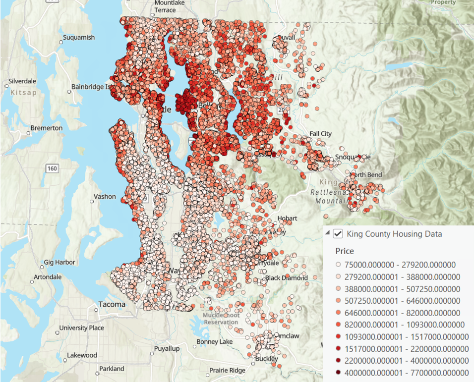
First, we will create a model to predict home price in the Forest-based and Boosted Classification and Regression tool.
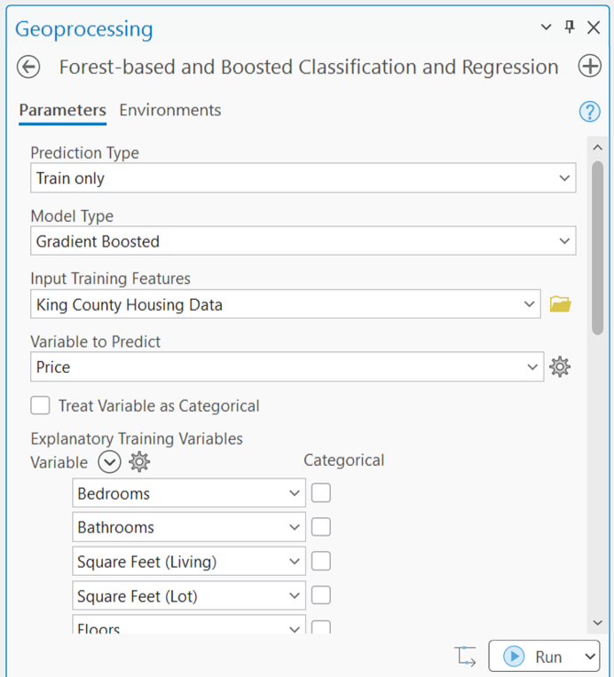
Be sure to save a Spatial Statistics Model File in the tool outputs!

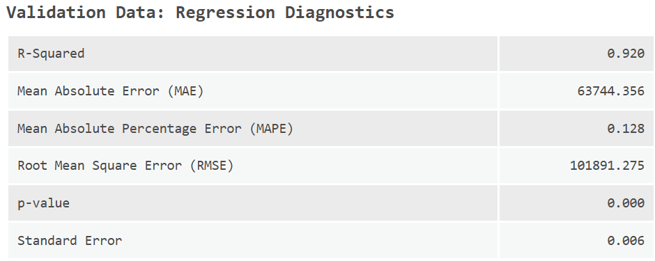
The validation R-squared is 0.92, meaning our model explains 92% of home price variation in leave-out data. Since we are confident in our model’s predictive ability, we can move into a post-hoc analysis to understand what each input variable is contributing to the prediction.
The fields used as explanatory variables are as follows:
- number of bedrooms
- number of bathrooms
- square feet of living area
- square feet of the lot
- number of floors
- whether the home is waterfront (0 to 2)
- condition of the home from 1 to 5, grade assigned to the home from 3 to 13
- square footage of the basement
- the year the home was built
- the latitude and longitude of the home
- the wildfire frequency surrounding the home
- land cover type surrounding the home
- tree canopy cover
- elevation
- terrain slope
This is an extensive list of explanatory variables, and it can be difficult to understand how an individual prediction gets generated by the algorithm with so many factors. This is where SHAP values will come in.
First, we will open the Evaluate Variable Influence for Predictions tool and input our Spatial Statistics Model File and select the new SHAP values Evaluation Type.
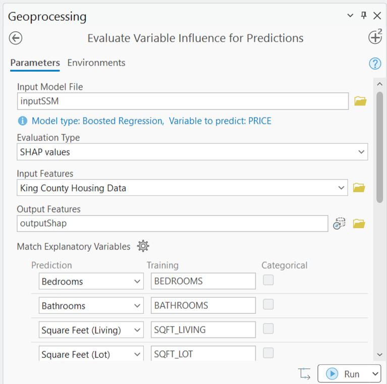
After running the tool, there are three primary outputs to consider and interpret. First, we will look at the output chart.
This chart is a new chart type called a beeswarm plot. It shows the distributions of a set of variables in your data. In this case, each row in the plot is a different set of SHAP values for the continuous explanatory variables in your model. Each point in a “swarm” represents one of the homes in our dataset.
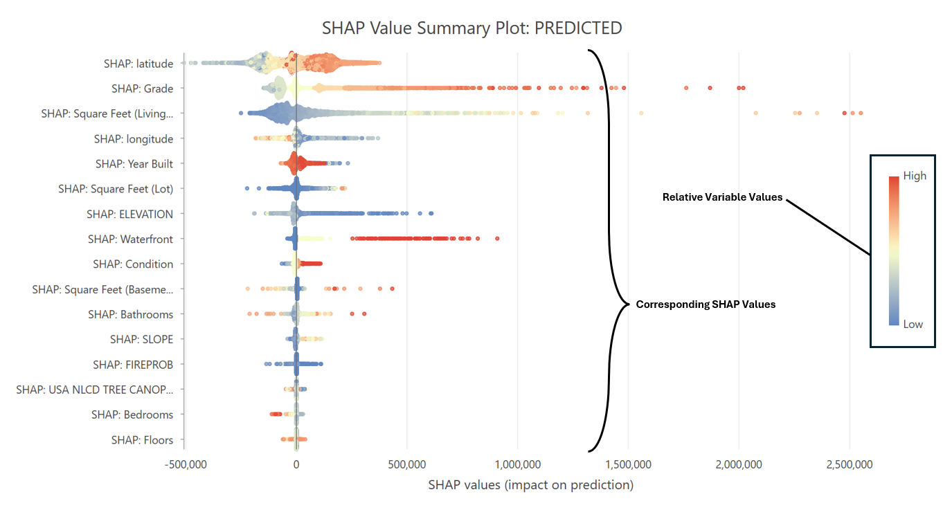
For the points to the right of 0, that particular variable led to an increase in the prediction. To help interpret this chart, we also have a color map that lets us compare the SHAP value to the original variable value.
For example, let’s look at the swarm for the variable at the top of the chart: latitude. The points to the right of 0 are red (high values of latitude), while the points to the left of 0 are blue and yellow (middle to low values of latitude). This tells us that a home being at a higher (red) latitude increases its price (positive SHAP value).
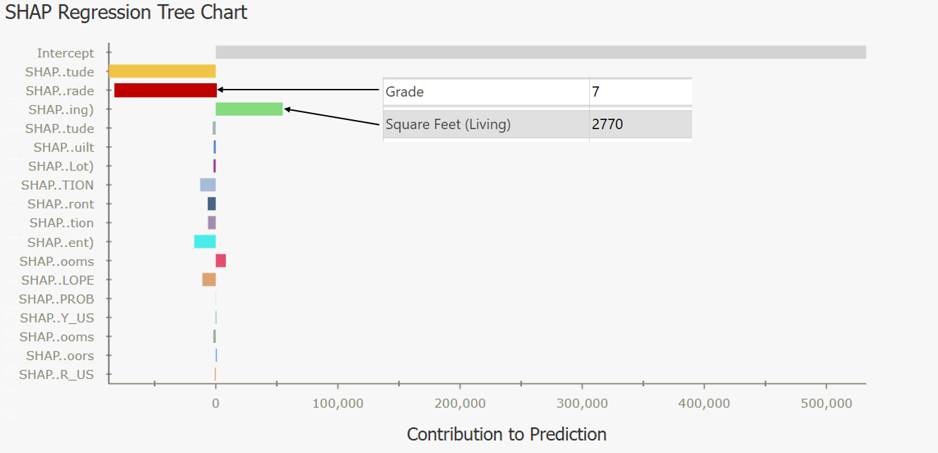
The next outputs are individual popup charts. After clicking on an individual home, we can see the breakdown of that home’s predicted price. In this first example, the Grade of the home was 7, which decreased the price (negative bar). The square footage was 2,770, and that value increased the predicted price of the home.
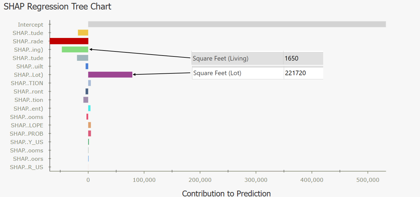
In this next example, the square footage of the home was 1,650, this value decreased the predicted price of the home. On the other hand, the property is 221,720 square feet, which significantly increased the predicted price.
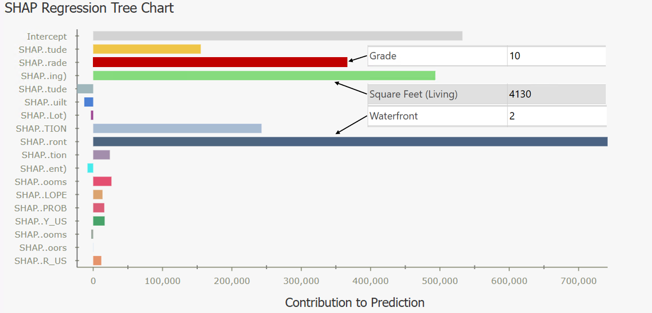
For this last example, we look at a very expensive home. It had a high Grade of 10, which increased the price. The square footage of the home was 4,130 which increased the price. And the home is on the waterfront, which significantly increased the predicted price. In this case, the largest bar is the dark blue Waterfront bar. The bar with the largest magnitude indicates the Key Variable, or the variable that influenced the predicted price the most.
Lastly, we will look at the symbology in the map. This map is symbolized by the Key Variable. As defined earlier, the Key Variable is the variable whose SHAP value has the largest magnitude (positive or negative), and therefore the largest influence on the predicted price at each individual location.
In the map, we can see more yellow points to the South, and yellow represents homes where the Key Variable was Latitude. So we can learn that in the southern part of King County, location is the most important factor for price.
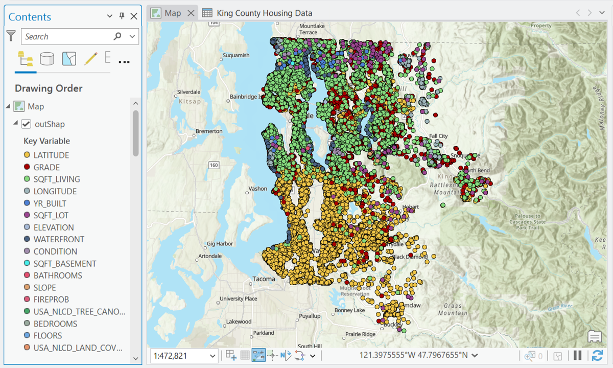
In the northern part of King County, we see more light green which indicates square footage as the Key Variable. Along the shorelines, we see the Waterfront variable symbolized, and as we get more rural toward the edges of the county, we can see the square footage of the lot being highlighted. This gives a regional view of variable importance, and is a new avenue to explore in spatial analysis.
This type of post-hoc analysis brings clarity to your predictive workflows. You can now:
- Explain individual model decisions to stakeholders.
- Identify regional trends and key drivers.
- Build trust in your spatial data science results.
In ArcGIS Pro 3.8, SHAP analysis is available for:
- Regression models (predicting continuous variables) created with the Forest-based and Boosted Classification and Regression (FBBCR) tool.
- Classification models (predicting categories) using gradient-boosted model types in the FBBCR tool.
Further Reading
King County home price prediction tutorials
Forest-based and Boosted Classification and Regression documentation
Article Discussion: