ArcGIS Pro 3.8 introduces Calculate Location Quotients, a new tool in the Spatial Statistics toolbox that helps identify areas with relatively high or low concentrations of a variable of interest compared to a meaningful benchmark. From employment and retail activity to health and education, the tool makes patterns of relative concentration easy to calculate, map, and explore.
Measuring relative concentration
The location quotient (LQ) is a foundational metric in regional science and economic geography that answers a key question for many spatial problems:
“Where is something more or less common than we would expect, compared to a larger region?”
Consider information sector jobs in the U.S. A map of employment counts shows where these workers are most prevalent in absolute terms.
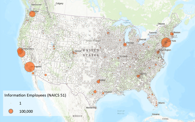
But many of these locations are also highly populated – so to what extent do the information sector jobs just reflect the large workforces in those areas? A rate provides more context by dividing information sector employment by total employment in each county. (Hint: use the Calculate Rates tool!)
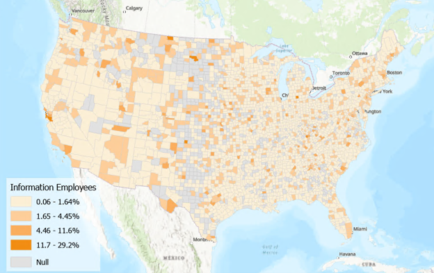
Now we can see where there are relatively higher and lower rates of information sector employment. But looking at one of these values on its own doesn’t help us understand its relative meaning: is 5 percent of employees working in the information sector a high or low amount? It’s hard to say without incorporating the broader regional context.
Location quotients do just that, by comparing this local share to a reference share. Here, the local share is the percentage of a county’s employees working in the information sector. For reference share, let’s consider the same percentage but for the country as a whole.
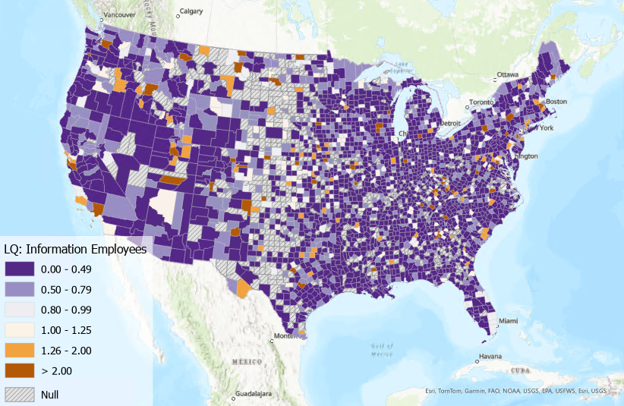
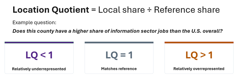
Dividing the local share by the reference share produces the location quotient, which is straightforward to interpret:
- An LQ of 1 means the local area matches the reference region.
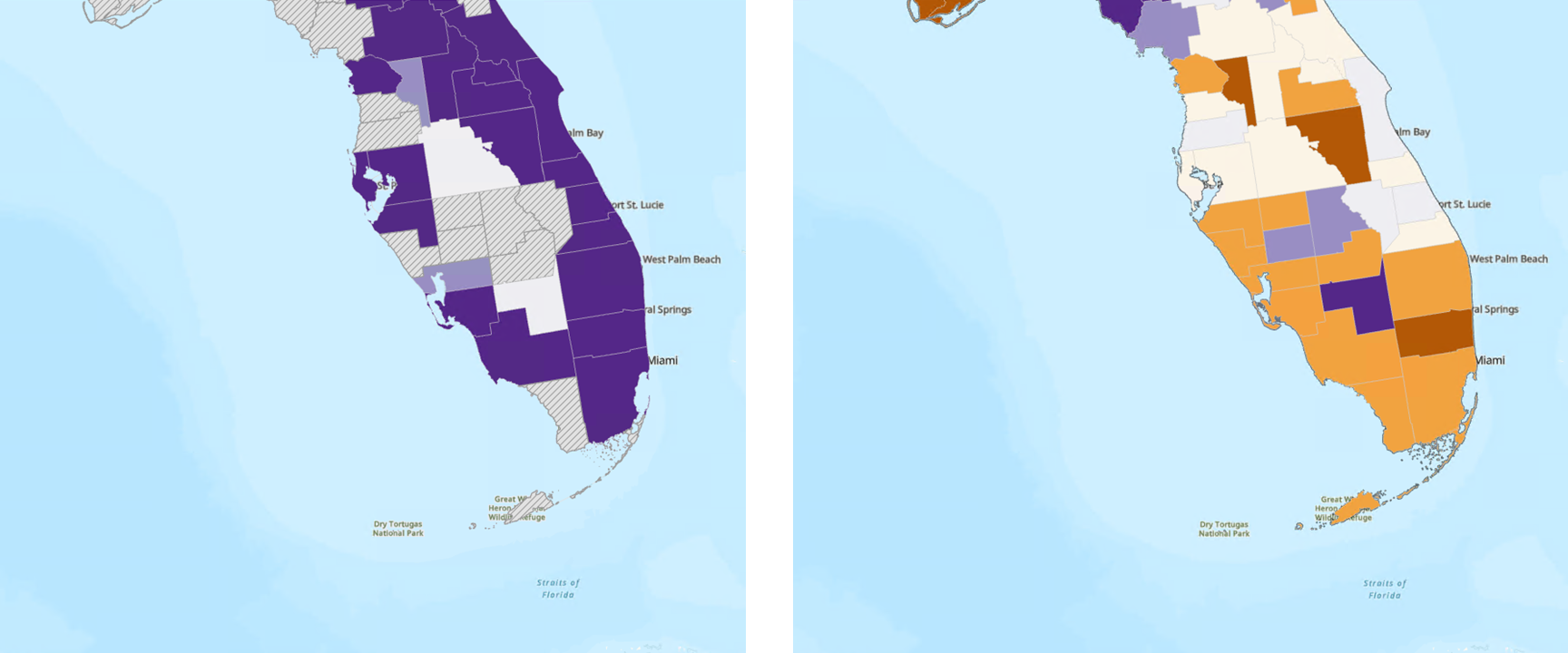
- Values less than 1 (purple) indicate relatively low concentration.
- Values greater than 1 (orange) indicate relatively high concentration.
For example, an LQ of 0.5 means the county has half the share of information sector jobs as would be expected based on the national rate. A county with an LQ of 2.0 has twice the expected share. LQ values that differ substantially from 1 indicate places that stand out relative to the benchmark – either because they are more concentrated or less concentrated than expected.
Comparing economic specialization profiles
LQs become especially useful when there are multiple categories of interest. Instead of just focusing on information sector jobs, LQs can be calculated for each of the 18 industries represented in the US Census Bureau’s County Business Patterns data.
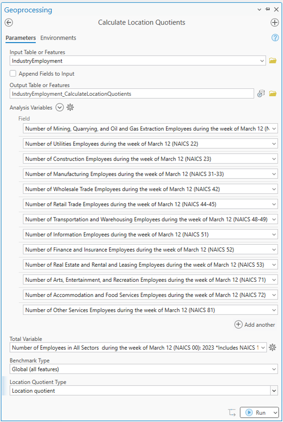
The output dataset contains a location quotient for every industry and every county, making it possible to compare specialization patterns across sectors. In South Florida, for example, employment in resource extraction generally has a lower relative concentration, while real estate employment has a higher relative concentration.
Exploring results with pop-ups
LQs can also be interpreted using pop-up charts created for each output feature. Clicking on a feature reveals the profile of LQs for that location, which can be compared against other features.
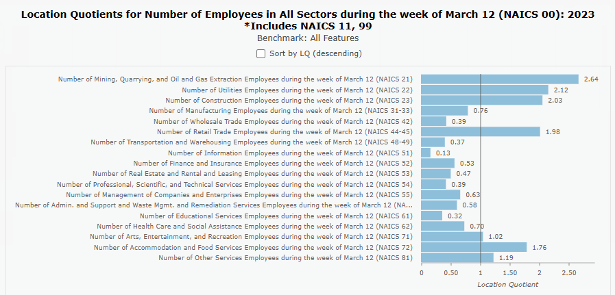
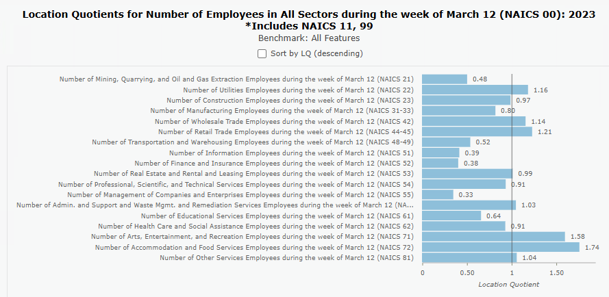
These pop-ups can be dynamically sorted to quickly reveal the categories with the highest and lowest relative concentrations in a location.
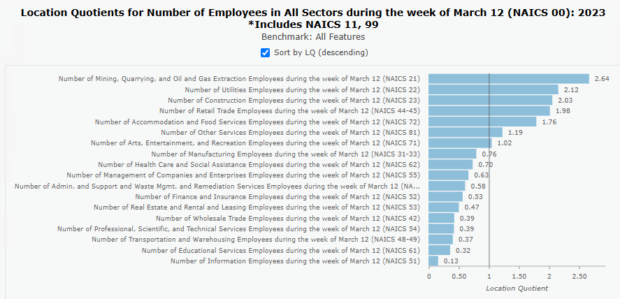
This makes it easier to compare places and identify the characteristics that distinguish them from surrounding regions.
Going beyond economic data
Although location quotients are commonly associated with industrial specialization, the method applies to far more than economic data.
In the example below, Chicago school data is used to examine the proportion of students eligible for free or reduced-price lunch. Instead of comparing every school to the citywide average, the analysis is stratified by charter status. The resulting map reveals spatial patterns in schools with relatively high and low levels of lunch eligibility, highlighting areas that stand out relative to comparable institutions.
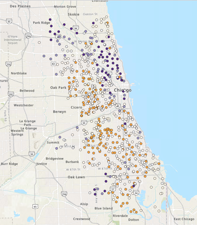
Alternatively, instead of deriving the benchmark from all or a subset of the input features, you can provide a known reference rate. This is useful when comparing to an established value, such as a statewide or national eligibility rate.
Interpreting results with charts
Calculate Location Quotients also creates charts to help with interpreting the results.
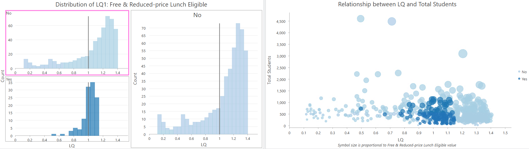
The output histogram shows the distribution and variability of the LQ and, when case groups are used, stratifies those distributions by group.
The output scatterplot provides context about observation size and potential outliers, helping to distinguish meaningful patterns from extreme LQs driven by small denominators.
Incorporating spatial neighborhoods
In addition to standard location quotients, the tool also supports focal location quotients (FLQs), which incorporate information from neighboring features into the calculation. By considering a feature and its neighbors together, FLQs can reduce the influence of highly localized variation and highlight broader patterns of concentration across a region.
Calculating your own location quotients
The new Calculate Location Quotients tool helps uncover patterns of specialization and relative concentration that can support decision-making across economic development, public policy, education, and many other fields. Learn more about this recent addition from the documentation, and we encourage you to try it out yourself!
Acknowledgements
Special thank you to Dr. Sarah Low (University of Illinois Urbana-Champaign) and Dr. Andrew VanLeuven (University of Vermont) for sharing their expertise and thoughtful feedback during the development of the Calculate Location Quotients tool.

Article Discussion: