See it first before diving in:
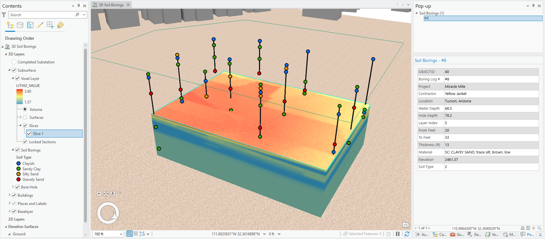
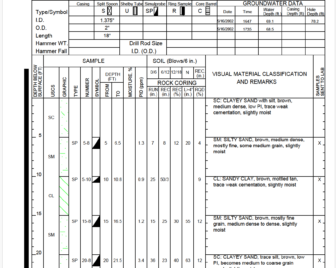
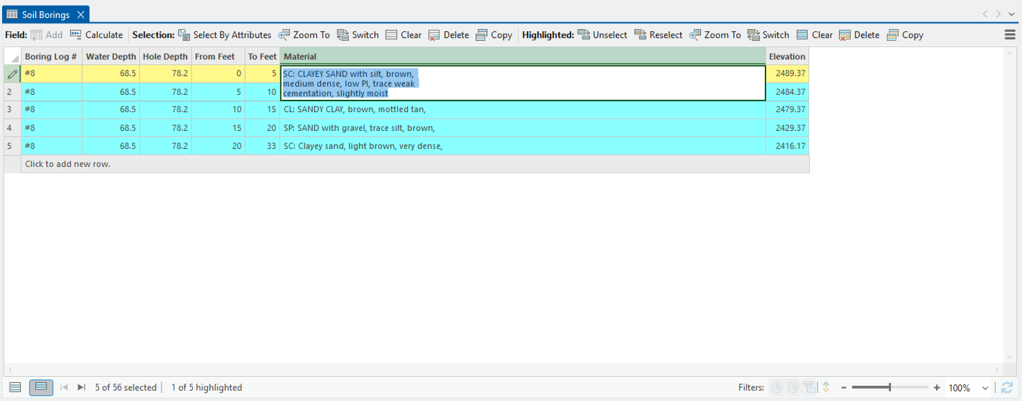
The image above shows a map of soil borings. Each point is a borehole log record, and each pop-up carries the full layer-by-layer profile of the core sample captured underground, classification codes, depths, field notes about cobbles and gravel, and where refusal occurred. None of them were typed in by hand. Every point was built by using a PDF boring log as input for an AI model running in ArcGIS Pro.
In this article, you will learn how to use a custom deep learning package (.dlpk) to build and modify a custom AI model. First, you’ll learn what this deep learning package contains and how it works.
A problem worth digging into
In geotechnical work, the boring log is one of the most information-dense documents in AEC, with a tight grid of depths, blow counts, recovery percentages, standard classifications, and terse field descriptions that were written next to a drill rig. A project might have dozens. A program might have thousands in a folder, scanned years ago and never looked at again.
The information in those logs is exactly what engineers need to understand ground conditions, but you cannot ask a folder of PDFs where the clay layers thin out or which borings hit refusal early. Someone has to open each file, read the column, and transcribe it by hand.
Every boring has a location and a vertical profile—a pure spatial signal—but a useful connection between that signal and a map requires manual data entry, time, and energy before it can inform a decision. Now you can use an AI model to read and process that data without leaving the geoprocessing environment, and you can build and modify that model to meet your needs.
The tool and the extensibility hook
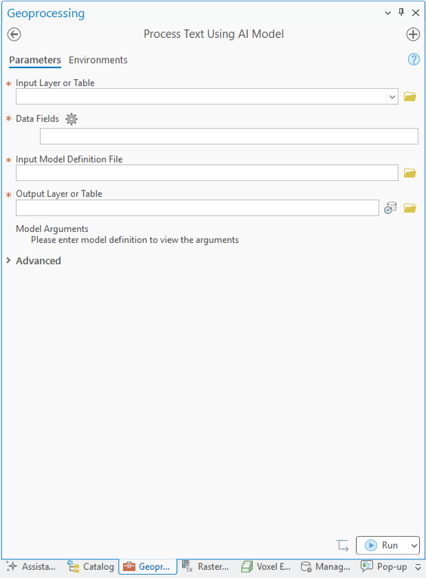
The ArcGIS Pro tool at the center of this workflow is the GeoAI toolbox and the Text Analysis framework for third-party language models. Rather than being limited to models trained directly in ArcGIS Pro, the framework allows Python developers to create a custom Natural Language Processing (NLP) function. This connects ArcGIS to an external language model, whether that is an open-source model or a commercial LLM exposed through a web API, and package that logic as an Esri deep learning package (.dlpk). That package then runs through the standard ArcGIS text analysis tools. In this case, that extensibility is what makes it possible to read geotechnical boring logs with a model that was not originally built inside ArcGIS.
Because the model uses a web API, the package is not tied to any one provider. It is compatible with Anthropic, OpenAI, Google Gemini, or Azure OpenAI, and the user running the tool chooses which one and supplies a key for it. Changing providers does not affect the extraction logic; it only changes which service the request is addressed to.
License: Using this capability requires the Advanced license level.
Caution: Only run Python and .dlpk files from a source you trust.
When you wrap a web-hosted LLM, the text you process is sent to that provider. Verify your data policy and your provider’s terms before using an LLM or AI tool.
Anatomy of a .dlpk file
A custom .dlpk file is a zipped folder containing an Esri model definition (.emd) file and the Python file that holds your inference logic. To create this .dlpk file, store the .emd and Python files in a folder with the same name as the .emd file name. Then compress it, and rename the zipped file to use the .dlpk extension.
In the .emd file, InferenceFunction names the Python file containing the logic, and ModelType communicates the type of task the model is designed to do. See the following example:
You can also run the package from an ArcGIS Pro notebook, which does not use the tool dialog box. Test on the version you intend to support.
In summary, the tool uses the information in the .emd file to access and process the code in the Python file.
Five methods that do the work
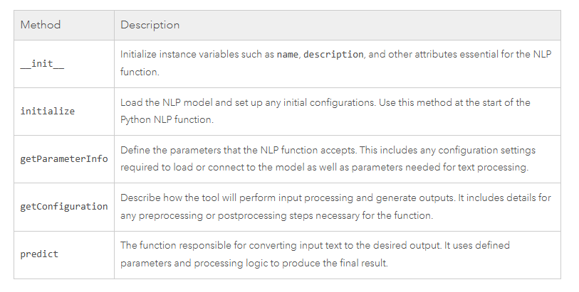
The inference function is a Python class, and the framework uses it to implement a small, predictable set of methods. Understanding these five methods is most of what you need to build or modify this AI model because they correlate to steps of a single tool run.
The constructor, __init__, sets identity. It names the class and provides a one-line description of what it does, which is extracting structured data from PDFs linked in a feature class.
initialize is where the model is loaded. It receives the path to the .emd file so it can read the configuration you stored there. For a locally loaded model, this is where the model’s trained weights (its numeric parameters) would be loaded. For this web-hosted model, there is little to load since it uses an API.
getParameterInfo is the method you will modify first when adapting this to your workflow. It defines the arguments the tool shows the user. Each parameter is a dictionary with a name, a data type, a default value, and whether it is required, and the tool turns that list into the model-arguments interface in the geoprocessing pane. The arguments a user sets at run time include the provider and a matching API key, which is supplied per run and never stored in the package. The arguments also include the model and its fallback, an endpoint for Azure, an optional page-chunk size for oversized PDFs, and optional overrides that use a different prompt or output schema on disk. The tool still uses the same patterns to build its model-arguments interface, but now it has more customization that does not require opening the .dlpk file.
getConfiguration runs after the parameters are known and sets up how the run will behave. This method reads which provider and model to call and its fallback, resolves the API key, and provides the right endpoint. You can choose Anthropic, OpenAI, Gemini, or Azure, and it supplies that provider’s endpoint, its authentication header, and the exact request and response shape that provider expects. The prompt, parsing, and output stay the same. getConfiguration also returns the batch size, which is the number of records the tool sends to the model at a time. You can modify this for your reports and rate limits.
predict is the engine. The tool sends it a FeatureSet of input rows and the name of the field holding the input, and it returns a FeatureSet of results. In this model, each input row points to a PDF, so predict encodes each PDF, sends it to the model with the extraction instructions, parses the structured response, and assembles the output, one row per soil layer. The shape you return here—the fields and their types—is exactly what appears in your output feature class.
Modify the package for your reports
What makes this package specific to boring logs is the extraction prompt and the output schema.
The extraction prompt communicates to the model the name of the input document and which data is requested. This is where geotechnical knowledge is stored, including the header fields, the per-layer classification codes, the depth intervals, and the descriptions. If you were using a different report type, such as environmental phase reports (for example, utility as-builts or inspection forms), you would rewrite this prompt to describe that document and its fields, and much of the rest of the script would carry over unchanged. The prompt is the domain expertise, written in plain language.
The output schema lists the fields the predict method builds into its returned FeatureSet. This determines what shows in your attribute table. When you add a field here and define how the parsed response fills it, it appears in the feature class. This also allows you to review your data for consistency and organization. For example, if a few depth fields carry meter labels in their aliases while the underlying values are in feet, that is the kind of unit-label mismatch a sharp geotechnical reviewer will catch. Aligning those is a quick and worthwhile task.
To further customize the package, you can also set the parameter list and configuration, the model you call, the fallback, and the batch size. However, these are optional because modifying the prompt and the schema allows you to retarget this package for a different set of documents without rebuilding the integration, which is the advantage of using a custom .dlpk file rather than a one-off script.
Putting it into production
A package that runs on your desktop is a proof of concept. Building it as a custom .dlpk file rather than a stand-alone script allows you to use it as more than a demonstration and integrate it into the rest of the ArcGIS system and your team’s workflows.
Boring logs are not standardized—a log from one firm can look nothing like another firm’s logs, and permits differ by jurisdiction. In production, you will need a small library of prompts, keyed to document type, and the tool must use the right one. The integration never changes; only the instructions do.
The next step is to increase the level of automation. Because Process Text Using AI Model is a geoprocessing tool, the workflow built around it can be published as a geoprocessing service to ArcGIS Enterprise and run on your server rather than a desktop. Once it is a service, it can be called on a schedule, triggered when new reports land in a watched location, or wired into a larger automated pipeline, so new logs added to a folder become mapped points without requiring you to open ArcGIS Pro. That is the difference between a tool a single analyst runs and a capability the whole organization relies on.
The Python inside the .dlpk file does not have to stop at returning a table. As code running in the geoprocessing environment, it can access the full ArcGIS API. That means the same package that reads the PDF can act on the extracted data. The package can publish a hosted feature layer, flag records that need human review, or write back into an existing dataset. The extraction and the action happen in one place. Instead of handing off a spreadsheet to another team, you can use the package to create a published, usable layer.
Tip: A single PDF of data that contains many boreholes can be more than the model can return in one answer, and the structured output comes back truncated. The page-per-chunk setting splits a large PDF into smaller page ranges, reads each on its own, and combines the records back together. Set it to about the number of pages one boring log spans, so a single hole is never cut across a boundary.
Accuracy
A confident wrong answer about subsurface conditions is worse than no answer. In testing, ten boring logs from a Tucson corridor project were run through the workflow. The test compared every extracted layer against the original PDF, building a frozen ground-truth file so the comparison could be repeated against any future change.
Across all ten boreholes, the soil layer sequence was correct every time, with the right classification codes in the right order, top to bottom. The layer count matched the log on all ten, including the busier profiles with six and seven distinct strata. And the total depth of each hole, where the sampler stopped or hit refusal, matched the log on all ten, down to the hundredth of a foot. Across 49 extracted layers, the stratigraphy and the codes were accurate to what the drillers recorded.
One header field, the site location, returned inconsistent values because these logs carry two different fields labeled location, a city and a named site, and the model often grabbed the city. That is not a model failure so much as an ambiguity in the source form, and the solution is a clearer line in the extraction prompt naming which location was intended. The extraction is only as unambiguous as the instructions you provide, and you find the ambiguities by checking the output against the source.

| Accuracy check | Result across all ten boreholes |
| Soil-layer sequence (classification codes, top to bottom) | Correct on all ten |
| Layer count per hole | Matched the log on all ten, including profiles with six and seven strata |
| Total depth (sampler stop or refusal) | Matched the log on all ten, to the hundredth of a foot |
| Total layers extracted | 49 layers, all faithful to what the drillers recorded |
| Site-location header field | Inconsistent — a source-form ambiguity, corrected in the extraction prompt |
That discipline is also how you handle a new log style. A form from a different firm may group its rows or name its classes in ways your prompt has not seen, and the first run will show you where. The fix stays in the prompt, not the integration: revise the instructions, use the new prompt without rebuilding the package, and check against the source until it matches. When you do that once per format, you build up a small library of prompts, each tuned to the layout it reads.
Automation supporting expertise
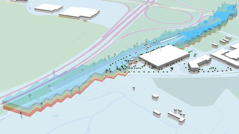
None of this replaces the geotechnical engineer or the boring log itself; the log is still the record. What the workflow adds is reach—decades of dense reports turned into interactive spatial layers that your team can view. Because every boring carries a location and its ordered stack of layers, the output geolocates automatically. When you symbolize by depth to refusal, dominant soil type, or whether groundwater was encountered, a corridor of scattered PDFs becomes a readable picture of ground conditions you can use in a dashboard, a web app, or a 3D scene. The data entry is automated, while the interpretation and decisions stay with the users.
If you have an archive of reports like this, your GIS team can transform those PDFs into actionable data visualization and map layers. Have questions, or want to share how you’d apply this?
Reach out to me on LinkedIn


Article Discussion: