Predicting where diseases may emerge is an impactful use of spatial data science. In this workflow, we will explore how new prediction evaluation enhancements in ArcGIS Pro can help produce more realistic and trustworthy models. Disclaimer: this blog is meant only for demonstrative purposes of new features in ArcGIS Pro.
The Challenge: Predicting to New Places
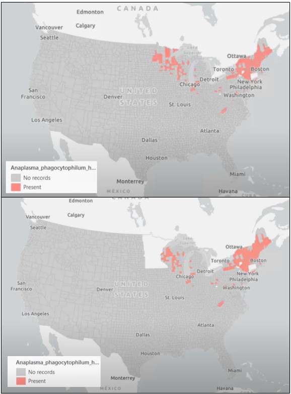
For this example, we will be studying the tick-borne illness anaplasmosis. Human anaplasmosis is transmitted by ticks and is unevenly distributed across the United States. For this analysis, we start with data for all U.S. counties from the CDC, but to simulate a realistic prediction challenge, we will intentionally exclude Minnesota from model training. This setup mirrors a common real-world scenario: we want to predict disease risk in a region where we don’t yet have confirmed observations.
Training an Initial Model
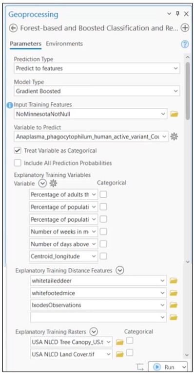
We begin by training a Gradient-Boosted model using the Forest-based and Boosted Classification and Regression tool. The model incorporates:
- Health and climate indicators from County Health Rankings
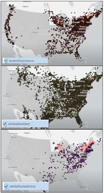
- iNaturalist observations of ticks
- iNaturalist observations of two mammal species known to carry the disease
- Land cover rasters
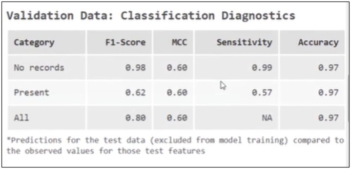
The tool automatically evaluates model performance using randomly selected hold-out data. At first glance, the results look reasonable:
Sensitivity is 57%, meaning the model correctly identifies a little more than half of counties with reported anaplasmosis that it has not seen during training.
Based on this metric, we would expect the model to identify roughly half of the affected counties when predicting into Minnesota.
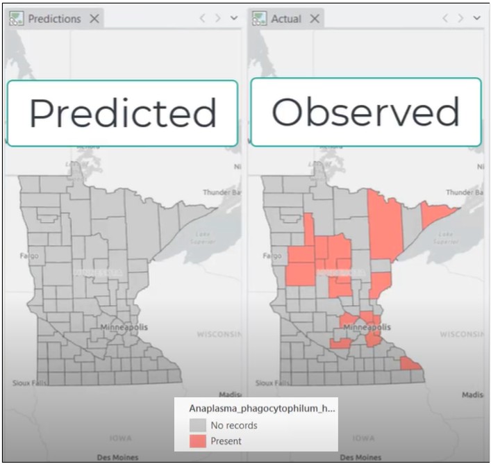
When we apply the trained model to Minnesota, the results are unexpected. The model identifies none of the known anaplasmosis counties.
So what happened? The reported performance suggested the model was adequate, yet it completely failed in a new spatial context.
What Went Wrong?
There are two issues at play.
1. Random Validation Can Inflate Performance
The initial evaluation used random validation, meaning training and test data were drawn from geographically similar areas. This allows the model to perform well on locations that closely resemble what it has already seen.
However, Minnesota represents a new spatial region, and random validation does not adequately test the model’s ability to generalize across space. Recall Tobler’s First Law of Geography: Everything is related to everything else, but near things are more related than distant things.
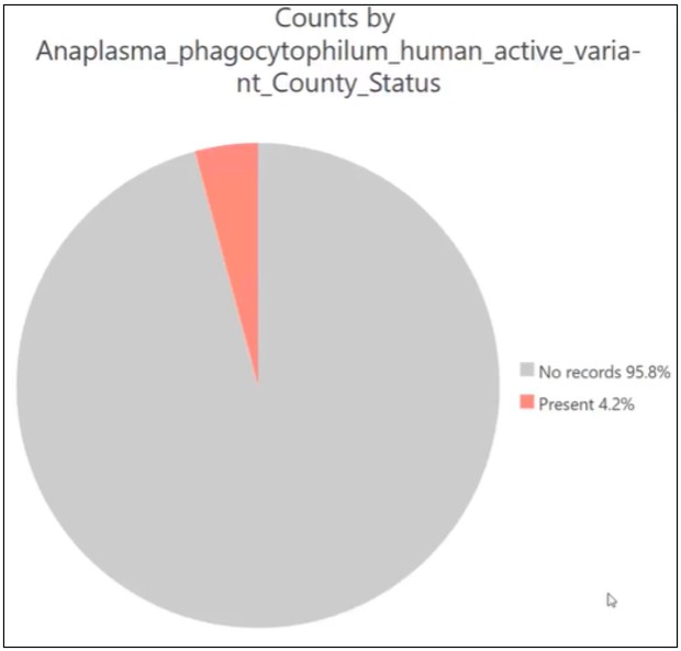
2. Anaplasmosis Is a Rare Event
Anaplasmosis occurs in a relatively small number of counties. This class imbalance makes it easy for a model to be overwhelmed by the majority (non-disease) counties and still appear accurate under standard evaluation metrics.
Improving Evaluation with Spatial Cross-Validation
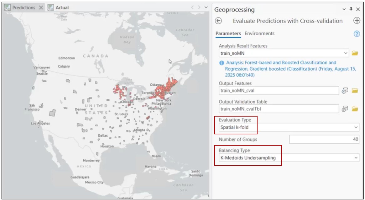
To address these issues, we turn to the Evaluate Predictions with Cross-Validation tool.
This tool introduces two critical improvements for rare, spatial phenomena:
Testing True Spatial Generalization
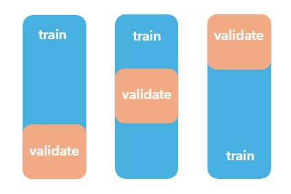
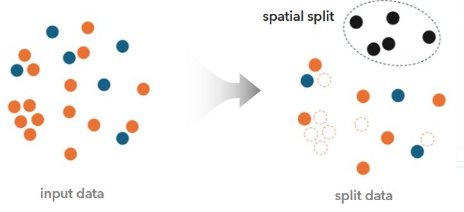
Instead of random splits, the tool performs spatial cross-validation, forcing the model to prove itself in geographic areas it has not encountered during training. This validation happens many times in many spatially contiguous areas to really test the model’s ability to generalize.
This produces a much more realistic estimate of how the model will behave when predicting into new regions.
Handling Rare Events with Undersampling
To prevent the model from being dominated by non-disease counties, we apply k-medoids undersampling. This balances the training dataset, so there are equal numbers of disease and non-disease counties for each validation run, while preserving the patterns in the data.
Note: Once you prove that balancing your data gives you reliable results, the Prepare Data for Predictions tool will help you take the necessary data engineering steps to balance data for training your final predictions.
Results That Match Reality
With these two factors in place:
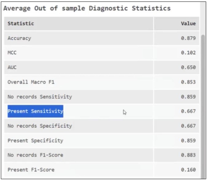
(1) Sensitivity improves to ~67% under spatial cross-validation
(2) When predicting into Minnesota, the model now correctly identifies about 60% of disease counties
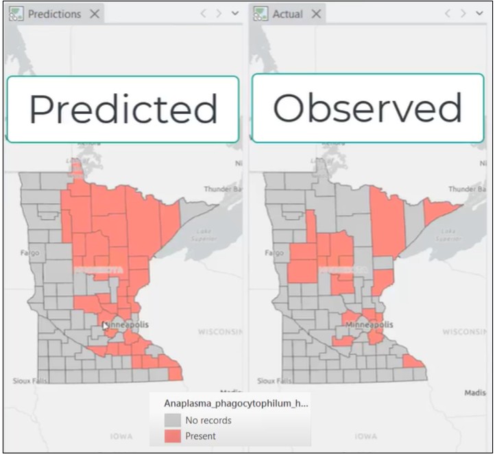
This alignment between reported performance and real-world prediction is exactly what we want to see.
Why This Matters
In most applied prediction problems, we don’t have “Minnesota data” waiting in the wings to validate our results. We must rely on model diagnostics to decide whether predictions can be trusted.
By accounting for spatial extrapolation and rare events, the new prediction evaluation tools in ArcGIS Pro provide performance metrics that reflect how models will actually behave in the real world. With accurate metrics come confidence, which is key when models are being used to inform decisions and policy.
Article Discussion: