Introduction
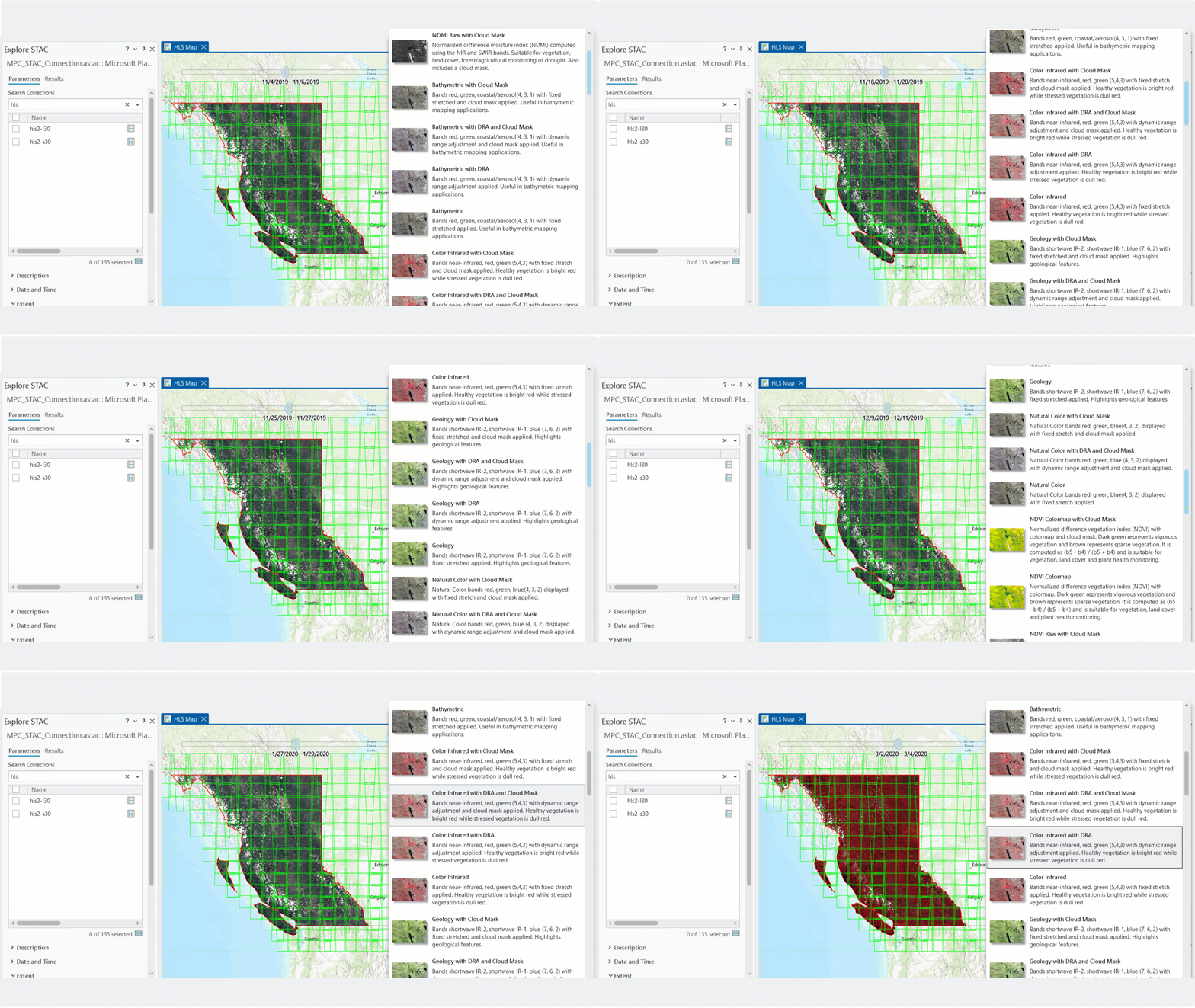
With the history and continuity of open missions for earth observation imagery, commercial cloud providers are hosting massive public data archives to empower scientific analysis of the earth through computing in their infrastructure. Examples include the Registry of Open Data on AWS and Microsoft Planetary Computer. Data available in these archives include a variety of imagery from a combination of platforms and sensors including ground-based, aerial, and satellite.
When paired with ArcGIS, a powerful set of capabilities emerge for gaining insight through imagery about earth’s natural and built environments. These applications include change detection, tracking annual vegetation growth cycles, and mapping natural disaster aftermath to name just a few.
Due to their global coverage and time span of consistent observations, some of the most widely used satellite collections arise from the set of Landsat and Sentinel-2 programs.
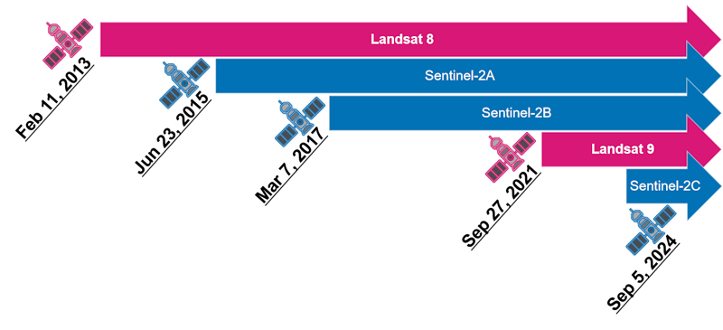
Landsat 1 was launched in 1972 and demonstrated high value in multispectral satellite imagery for land-resource monitoring. This provided the technical and scientific foundation for Landsat missions 2 through 9, with Landsat 8 and 9 still operating in 2026. Landsat 8 was launched in 2013 providing 16-day revisit cadence. Landsat 9 launched in 2021 with its own 16-day revisit cadence. Together, Landsat 8 and 9 provide global coverage with an 8‑day revisit interval for the same location on Earth.
Sentinel-2A was launched in 2015 and was followed by Sentinel-2B in 2017 to achieve a 5-day equatorial revisit capability. In 2024, Sentinel-2C was launched for mission continuity and to replace Sentinel-2A after extended service period. In 2026, all three satellites are still operational and providing even greater (3.3 day) revisit capability.
In addition to varied temporal resolution, these missions offer similar multispectral, and in the case of Landsat, thermal capabilities. They also offer varying spatial resolutions across the sensor spectral bands. These sensors aboard the five satellites include Landsat Operational Land Imager (OLI) and Sentinel-2 Multispectral Imager (MSI).
What if analysis requires greater revisit than possible within Landsat or Sentinel-2 alone? That’s where the power of harmonization comes into focus. Harmonization is a process that can bring these similar, yet unique data sources together into a new, more powerful unified source.
This article walks through how to access, manage, and analyze Harmonized Landsat Sentinel-2 (HLS) data in ArcGIS, and demonstrates a repeatable workflow for generating cloud-free composites and analyzing natural phenomena over time.
Harmonized Landsat Sentinel-2
NASA, led by NASA Goddard Space Flight Center, in collaboration with the U.S. Geological Survey and the European Space Agency developed the HLS dataset. This demonstrated that Landsat 8 and Sentinel‑2 surface reflectance data could be physically harmonized and used together as a single, analysis‑ready time series at 30 m resolution, enabling near‑daily land surface monitoring while preserving radiometric consistency. This initial HLS version was first released publicly in 2018 with limited spatial coverage (primarily North America and select regions). The superset of HLS imagery is split into two constituent datasets, HLS Landsat (HLSL) and HLS Sentinel-2 (HLSS).
In 2021, HLS v2.0 was released providing global land coverage (excluding Antarctica) with updated and improved harmonization algorithms, and historical processing of the archive was completed in 2023. This version shifted to the Landsat Collection 2 ground control points, improving geolocation using Sentinel-2 Global Reference Image as the absolute reference. Improved atmospheric correction and harmonization algorithms were used and version 2.0 also introduced Cloud Optimized GeoTIFF (COG) format files supporting cloud-native workflows. Version 2.0 also included Sentinel-2C for the first time. Together, these improvements transitioned from experimental, regional coverage to operational global production.
In September 2023, HLS v2.0 was made available within the NASA Earthdata Cloud archive (LPCLOUD) as part of the Land Processes Distributed Active Archive Center (LP DAAC) and included in NASA’s Common Metadata Repository (CMR), empowering search and discovery using SpatioTemporal Asset Catalog (STAC).
This virtual constellation includes five satellites across the Landsat and Sentinel-2 programs.

Together, these satellites provide an enhanced temporal period spanning a continuous archive from Feb 11, 2013 to the present day. Additionally, they enhance temporal resolution by providing a higher revisit rate than any single satellite program and reaching the highest global mean effective revisit rate of ~1.4 days during coverage of all five satellites.
Harmonization
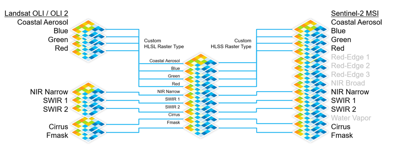
Harmonization of the HLS imagery sources involves spatial, spectral, and radiometric resolutions.
Spatial resolution is harmonized from a variety of 10-, 20-, and 60-meter bands of MSI, to match the consistent 30m bands of OLI.
Spectral resolution is harmonized from subtle differences in the spectral wavelength bands of MSI and OLI.
Radiometric resolution is harmonized by normalization of illumination, view angle, and dynamic range to 16-bit.
The convergence of this harmonization produces a consistent spatial, spectral and radiometric product having eight multispectral bands common to both Landsat and Sentinel-2 products, plus a quality band (FMask) indicating areas of the highest quality pixels defined by atmospheric conditions including clouds and aerosol level. See table below for details.
| Band name | OLI band number | MSI band number | HLS band code name L8/L9 | HLS band code name S2 | Wavelength (micrometers) |
| Coastal Aerosol | 1 | 1 | B01 | B01 | 0.43 – 0.45 |
| Blue | 2 | 2 | B02 | B02 | 0.45 – 0.51 |
| Green | 3 | 3 | B03 | B03 | 0.53 – 0.59 |
| Red | 4 | 4 | B04 | B04 | 0.64 – 0.67 |
| NIR Narrow | 5 | 8A | B05 | B8A | 0.85 – 0.88 |
| SWIR 1 | 6 | 11 | B06 | B11 | 1.57 – 1.65 |
| SWIR 2 | 7 | 12 | B07 | B12 | 2.11 – 2.29 |
| Cirrus | 9 | 10 | B09 | B10 | 1.36 – 1.38 |
| FMask | – | – | FMask | FMask | – |
Converging Common Bands
While OLI and MSI sensors present some unique bands, the majority (Red, Green, Blue, NIR Narrow, SWIR 1, SWIR 2, and Cirrus) are measured by both.
HLS Benefits
Applications of raster analysis requiring high temporal resolution are ideal candidates for the HLS v2.0 data. Some notable examples include forest or crop health assessments since the progression of change can be critical in the efficacy of potential actions prescribed by analysis.
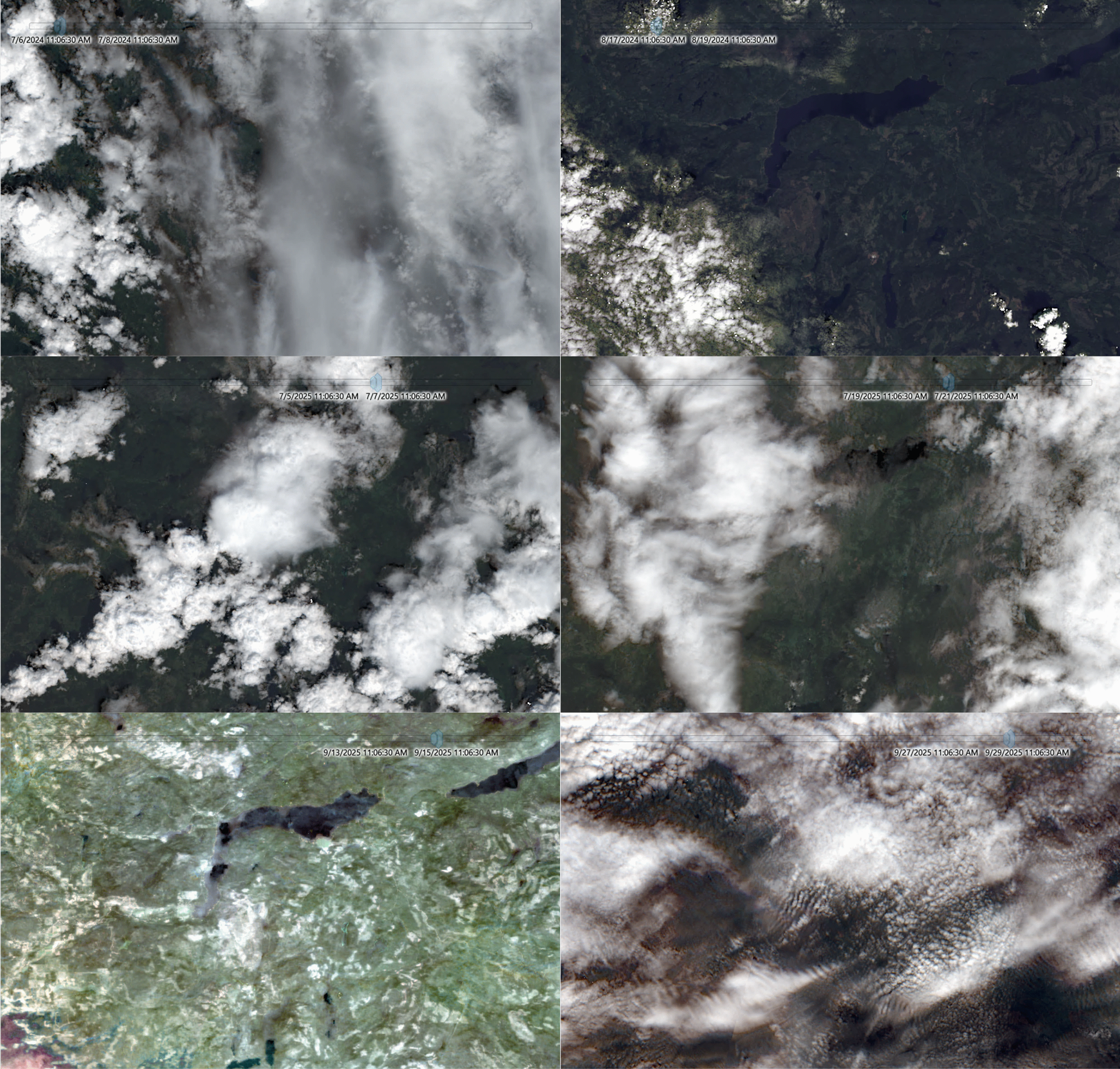
Another advantage of using the HLS v2.0 data is the ability to produce cloud-free composites through map-reduce aggregation methods in ArcGIS.
Access and Management
This section deals with how to operationalize HLS v2.0 in ArcGIS, from accessing the cloud-hosted imagery to managing it in a mosaic dataset.
GitHub Repository
A public GitHub repository is available at https://github.com/dkwright/arcgis-nasa-earthdata to further describe and automate the methods in this article.
This repository contains a variety of resources to help create mosaic datasets from precise sets of HLS v.20 imagery that are accessed using the NASA Earthdata CMR STAC API. These resources include:
- Python notebooks to automate the creation of ArcGIS Cloud Storage (ACS) connection files for accessing HLS v2.0 data in the NASA Earthdata AWS environment
- Custom ArcGIS raster types for easy management of the HLS Landsat and HLS Sentinel-2 imagery in NASA Earthdata AWS, or Microsoft Planetary Computer environments
- ArcGIS raster function templates for a large variety of on-the-fly rendering of band composites, band indices, with and without cloud-masking in NASA Earthdata AWS, or Microsoft Planetary Computer environments
ArcGIS Cloud Storage Connection Files
ArcGIS users can access imagery in cloud storage directly using ACS connection files with ArcGIS Pro and cloud stores with ArcGIS Server. These access conventions support visualization and analysis of imagery located in cloud object storage. The HLS v2.0 data can be accessed in the NASA Earthdata source in AWS, as well as the Microsoft Planetary Computer.
When accessing cloud-optimized imagery from cloud object storage, efficient ranged requests are possible, improving performance and limiting the amount of data transmitted from cloud storage to ArcGIS to just the extent and scale being requested. For ad-hoc visualization and staging raster analysis, the ArcGIS Pro client can technically be on any machine anywhere. However, for production analysis on appreciable scale, the ArcGIS Pro machine should be deployed as a virtual machine in the same region of the same cloud. Pairing compute with data in the same cloud and region is a best practice for maximizing performance and reducing data egress.
Working with HLS v2.0 in AWS
To access HLS v.20 imagery from NASA Earthdata, a free NASA Earthdata account is required and can be created at: https://www.earthdata.nasa.gov/data/earthdata-login.
ArcGIS makes use of these credentials in ACS connection files for ArcGIS Pro, and can also be used in an Image Server cloudstore definition.
The NASA Earthdata HLS v2.0 products are located in AWS region us-west-2 (Oregon). There are two methods for creating ACS connection files for HLS v2.0 data access in ArcGIS Pro. The first method is by setting the ACS Service Provider to WEB. This WEB method sets up data access over HTTPS protocol and can be used on any computer with an internet connection. If you’re getting familiar with the HLS v2.0 data, doing some visualization with raster function templates, or building/validating an analysis workflow, this method works well. In the GitHub repository, use /notebooks/NASA_Earthdata_ACS_Creator_Web.ipynb to build your ACS connection file.
The second method sets the ACS Service Provider to AMAZON. This method establishes data access using the S3 protocol and in the case of NASA Earthdata, requires ArcGIS Pro is running on a virtual machine in AWS Elastic Compute Cloud (EC2) within the us-west-2 (Oregon) region – co-located with the HLS v2.0 data. If you’ve already honed your analysis workflow, are pursuing analysis at large scale, or simply want the fastest possible configuration this method is ideal.
Working with HLS v2.0 data in Microsoft Planetary Computer
The Microsoft Planetary Computer HLS v2.0 products are located in Azure region westeurope (West Europe) and ACS connection files are available in the ArcGIS for Microsoft Planetary Computer public GitHub repository https://github.com/Esri/arcgis-for-mpc.
Within the repository, there are two ACS connection files that are required for accessing the HLS v2.0 data:
- AMPC_Resources/ACS_Files/esrims_pc_hls2-l30.acs
- AMPC_Resources/ACS_Files/esrims_pc_hls2-s30.acs
Analysis: Monitoring Forest Moisture Conditions
Study Area and Dataset Overview
This case study demonstrates one way ArcGIS can be used to support forest health monitoring using the HLS v2.0 imagery. The example focuses on deriving cloud-free multispectral monthly summer composites and using the Normalized Difference Moisture Index (NDMI) to explore spatial and temporal patterns related to forest moisture conditions.
The study area is located in British Columbia, Canada, a region characterized by complex terrain, diverse forest ecosystems, and frequent cloud cover. These conditions make consistent optical analysis challenging, particularly when single-sensor imagery may not provide enough clear observations.
To support seasonal comparison, the analysis focuses on summer observations collected between July and September from 2024 to 2025. Restricting the analysis to the same seasonal period helps reduce variability associated with vegetation phenology and improves comparability between years.
Building the Cloud-Free Summer Compositing
Workflow
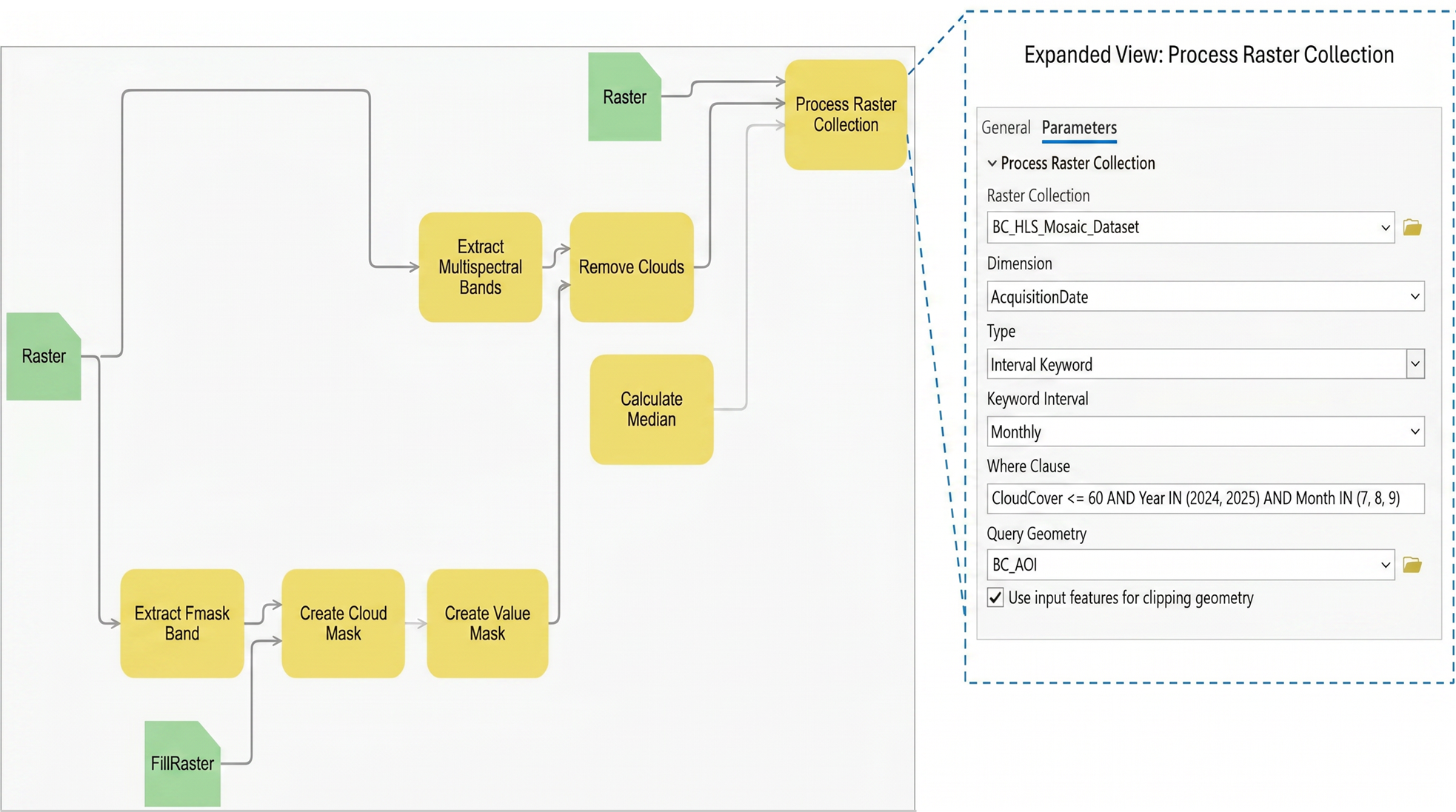
Cloud-free monthly composites are generated from the HLS imagery collection using a raster function template in ArcGIS. The raster function template used in this example is available for download from the GitHub repository introduced earlier, allowing you to reproduce or adapt the workflow for your own HLS analyses.
The workflow consists of the following image processing steps:
- Extract multispectral bands: The Extract Bands raster function isolates the seven HLS surface reflectance bands required for analysis
- Create cloud mask: The Fmask quality band is extracted, cloud-contaminated pixels are identified, and a binary cloud mask is generated using the Extract Bands, Transpose Bits, and Boolean Not raster functions, respectively
- Apply per-pixel cloud removal: The Clip raster function applies the cloud mask to the surface reflectance bands, removing cloud-contaminated pixels while preserving valid observations
- Filter and composite imagery: The Process Raster Collection function follows a map–reduce workflow. The map stage applies steps 1–3 at the pixel level for each raster in the collection, while the reduce stage performs image selection and aggregates the results into monthly composites, as follows:
- Filter the imagery collection using the following expression: CloudCover <= 60 AND Year IN (2024, 2025) AND Month IN (7, 8, 9). This limits the analysis to summer observations with acceptable cloud conditions. These parameters can be modified based on the study area and monitoring objectives
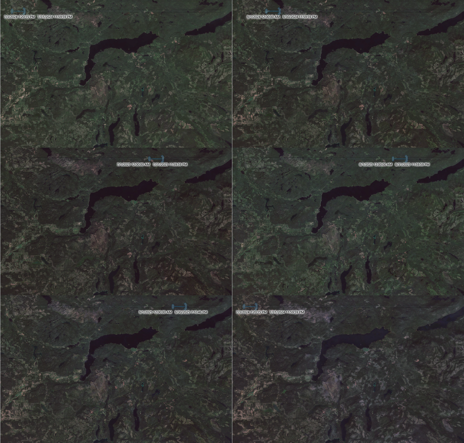
- Aggregate valid observations into monthly cloud-free composites using the Geometric Median raster function. Median compositing minimizes the influence of residual clouds, cloud shadows, and anomalous reflectance values
The workflow produces a consistent monthly summer time series of composites for each year, derived from only cloud-filtered observations. These composites serve as analysis-ready inputs for downstream applications, where temporal consistency and reduced atmospheric contamination are critical for reliable comparison across seasons and years.
Deriving Normalized Difference Moisture Index (NDMI): Forest Moisture Indicator
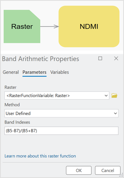
Forest moisture condition is assessed by computing the NDMI directly from the cloud-free monthly multispectral composites. NDMI leverages the differential sensitivity of near-infrared and shortwave infrared reflectance to leaf water content, making it a well-established proxy for canopy moisture stress in forested landscapes.
In ArcGIS, NDMI is calculated using the Band Arithmetic raster function. The index is generated dynamically from the composite imagery, allowing the same calculation to be applied consistently across each time step without creating intermediate raster datasets.
The NDMI formula:
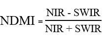
- Band 5 — Near-Infrared (NIR) ~865 nm
- Band 7 — Shortwave Infrared (SWIR) ~2130 nm
NDMI values range from −1 to +1:
- Higher positive values indicate relatively higher canopy moisture
- Lower values may indicate increasing moisture stress or drought conditions
Explore Spatial and Temporal Forest Health Patterns
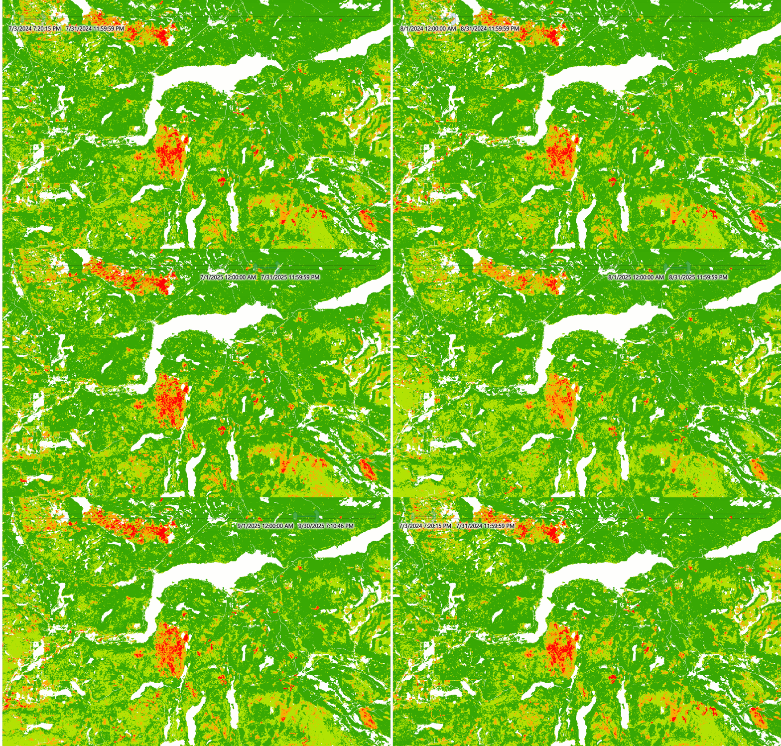
The NDMI output is filtered to forested areas using a land use/land cover (LULC) layer derived from the HLS cloud-free composite and a pretrained deep learning model. The resulting NDMI values are symbolized using a consistent color ramp.
An animation of the summer monthly NDMI from 2024 to 2025 is used to visualize temporal change. The time slider in ArcGIS Pro enables continuous playback of the dataset, making it easier to observe patterns of increasing or decreasing moisture over time.
This temporal view supports time series analysis of forest moisture conditions, revealing areas with persistently low NDMI (indicative of chronic stress), locations with year-over-year variability driven by climate fluctuations, and spatial clustering patterns associated with environmental factors such as elevation and aspect.
Insights for Forest Health Monitoring
This example illustrates how analysis-ready, harmonized imagery combined with raster functions and time-aware visualization in ArcGIS supports efficient forest health assessment. Cloud-free composites provide a stable foundation for seasonal comparison, while NDMI offers a relative indicator of forest moisture condition across space and time.
Observed patterns are influenced by forest type, elevation, aspect, and climate variability, reinforcing the importance of interpreting NDMI in environmental context. More broadly, this workflow demonstrates just one of many analytical pathways supported by ArcGIS. The same imagery and processing approach can be extended to additional industries, health indicators, longer time series analysis, zonal summaries, and integration with dashboards and web applications for monitoring and decision support.
Conclusion
This article demonstrates how ArcGIS operationalizes cloud-hosted HLS imagery through an end-to-end workflow spanning data access, management, analysis, and time-enabled visualization.
Although the example is implemented over a focused study area and time period, the same approach can be applied across a wide range of environmental monitoring applications and readily scaled to larger geographic extents and higher data volumes.
HLS imagery uniquely addresses the need for temporally dense measurements when earth surface conditions are changing rapidly, and especially in persistently cloudy geographies and climates. This benefit is even more advantageous when the need for seasonal composites are selected for analysis because the time range is compressed.


Article Discussion: