For many users, the Vector Tile Style Editor (VTSE), or editing the style extracted from a vector tile package, has long been a way to change static style properties such as colors, fonts, and symbol sizes. See ‘Restyling Vector Tiles’ to learn how.
Some customers use this method to add vendor-specific functionality to their vector tile styles, and now we are introducing wider support for Mapbox and MapLibre style expressions. From the 3.8 release, ArcGIS Pro can natively consume and render vector tile packages that contain expressions, extending support to desktop workflows. Expressions are currently authored within the vector tile style JSON file, though VTSE provides several graphical interfaces to help.
Building smart map styles
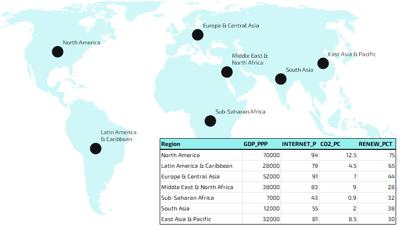
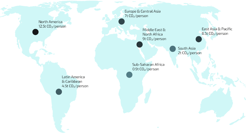
I’m using vector tiles from my previous post on the basics of restyling vector tiles. These are a circle symbol on a center-point I generated for each of the world regions as per data from World Bank, as seen above.
I’m going to use the various fields and attributes from my estimated demographics dataset to drive updates to the map symbology.
Let’s open the style JSON and begin.
Pro Tips: If using Create Vector Tile Package tool, use the highlight option on the attribute table in Pro to ensure all the fields you want are available to the vector tile style.
Consider using the Vector Tile Style Editor (VTSE) in ArcGIS Online and ArcGIS Enterprise as a visual sandbox to quickly try out changes and expressions.
Example 1: Internet Access
Expressions can make decisions.
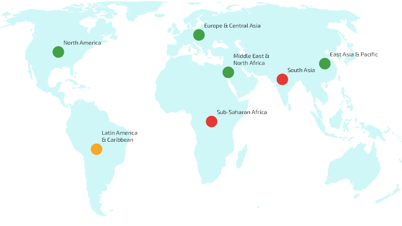
I’m going to use an expression to replace my static black circle color and to decide whether my region circles should be red, amber or green.
Say green is 80% or more have access to internet, amber is 70% to 80%, and less than 70% is red.
I’m going to edit this section of the style JSON:
{
”id”: “world_bank_regions_demo”,
”type”: “circle”,
”source”: “esri”,
”source-layer”: “world_bank_regions_demo”,
”layout”: {},
”paint”: {
”circle-radius”: 12,
“circle-color”: “#131315”
}
}
Specifically, I’ll replace the static circle-color with the following expression:
“circle-color”: [
”case”,
[
”<“,
[“to-number”, [“get”, “INTERNET_P”]],
70
],
”#e53935″,
[
”>=”,
[“to-number”, [“get”, “INTERNET_P”]],
80
],
”#43a047″,
”#f9a825″
]
Example 2: World Regions
Expressions can map categories to styles.
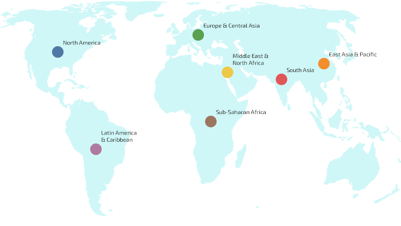
I’m going to use an expression to assign desired color values to each circle based on the region from the data, to apply a custom harmonized palette.
So, I will replace:
“circle-color”: “#131315”
With:
“circle-color”: [
”match”,
[“get”, “Region”],
”North America”, “#4E79A7″,
”Europe & Central Asia”, “#59A14F”,
”East Asia & Pacific”, “#F28E2B”,
”South Asia”, “#E15759″,
”Sub-Saharan Africa”, “#9C755F”,
”Latin America & Caribbean”, “#AF7AA1″,
”Middle East & North Africa”, “#EDC948″,
”#AAAAAA”
]
Example 3: Gross Domestic Product (GDP)
Expressions can scale symbols continuously based on data values.
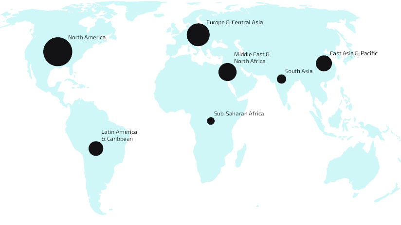
I’m going to use an expression to interpolate to vary and assign circle symbol size based on the GDP (PPP) values from the data compared to a minimum and maximum symbol size.
So, this time I will replace:
“circle-radius”: 12
With:
“circle-radius”: [
”interpolate”,
[“linear”],
[
”get”,
”GDP_PPP”
],
7000,
8,
70000,
30
]
However, variable symbol sizes will overlap our static offsets for text, so I will also replace:
“text-offset”: [
0.875,
-0.875
]
With:
“text-radial-offset”: [
”interpolate”,
[“linear”],
[
”get”,
”GDP_PPP”
],
7000,
0.75,
70000,
2.5
]
The best approach for adjusting label placement will depend on the map and the properties supported by your renderer.
Example 4: Carbon Dioxide Emissions
Expressions can calculate and format information dynamically.
I’m going to use an expression to create dynamic labels from field values using the concat (concatenate) function. This will clearly label each region of the map with its Carbon dioxide (CO₂) emissions per capita, measured in metric tonnes per person per year. Other functions such as to-string, round, and divide can be combined to format values or convert them into more meaningful units before they are displayed.
So, I will replace:
“text-field”: “{_name}”
With:
“text-field”: [
”concat”,
[
”get”,
”Region”
],
”\n”,
[
”get”,
”CO2_PC”
],
”t CO₂/person”
]
I also made some minor adjustments to size, color and anchor properties.
Example 5: Making less of a point
Expressions can react to map scale.
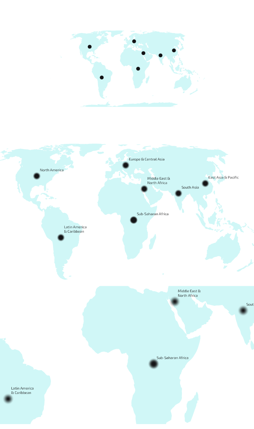
I’m going to add a blur to my circles and use an expression to dynamically change the size of that blur as I zoom in and out between levels. I’ll use a similar interpolate technique to subtly control the circle-size to support the blur, and as before will change the static text-offset to a dynamic text-radial-offset to maintain clear label placement across scales.
So the main story here is that I add:
“circle-blur”: [
”interpolate”,
[“linear”],
[“zoom”],
0,
0,
2,
1
]
At small scales the symbols remain crisp and understated, helping to preserve a clean overview. As users zoom in, the increasing blur and subtle growth in symbol size give the regions a good balance of greater visual prominence with less geographic precision. After all, these are representations of large polygonal regions rather than precise point locations.
Example 6: Renewable Energy (zoom + property)
Expressions can adapt styles across scales and increase thematic emphasis as users zoom.
At a global view, the goal is to highlight patterns, not overwhelm with detail. Even at small scales, a map often benefits from gradually introducing new information as users zoom in. Style expressions can help adjust visual hierarchy and content as users explore different scales.
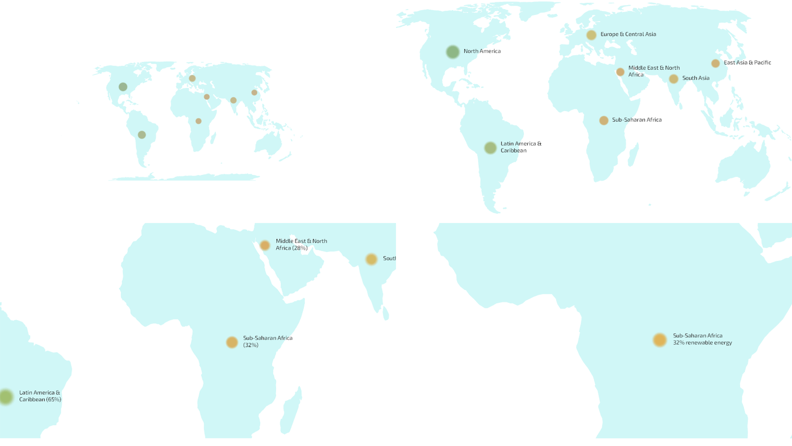
In this example, I’ll combine zoom level and the proportion of each region’s energy generated from renewable sources to create a style that evolves across scales. Symbols become more prominent, regional differences become easier to distinguish, and labels emerge as the thematic story comes into sharper focus.
So, I will set circle-radius as:
“circle-radius”: [
”interpolate”, [“linear”], [“zoom”],
0,
[
”interpolate”, [“linear”], [“get”, “RENEW_PCT”],
0, 4,
100, 10
],
3,
[
”interpolate”, [“linear”], [“get”, “RENEW_PCT”],
0, 9,
100, 37
]
]
Renewable energy differences become more visible as the map scale increases.
I will set circle-color as:
“circle-color”: [
”interpolate”, [“linear”], [“zoom”],
0,
[
”interpolate”, [“linear”], [“get”, “RENEW_PCT”],
0, “#A98692”,
25, “#C4B18F”,
50, “#C2C095”,
75, “#9EB697”,
100, “#7AAEA7″
],
3,
[
”interpolate”, [“linear”], [“get”, “RENEW_PCT”],
0, “#C65D7B”,
25, “#E3A857”,
50, “#D8D45B”,
75, “#79B96D”,
100, “#2AA7A1”
]
]
Now high-renewable regions don’t just get bigger. They become visually dominant.
Putting It All Together
We’ve looked at expressions individually, but their real power comes from combining them. This short walkthrough demonstrates a more complete styling story, using expressions to drive symbol size, color, and progressively richer, localized labels for a global airports dataset.
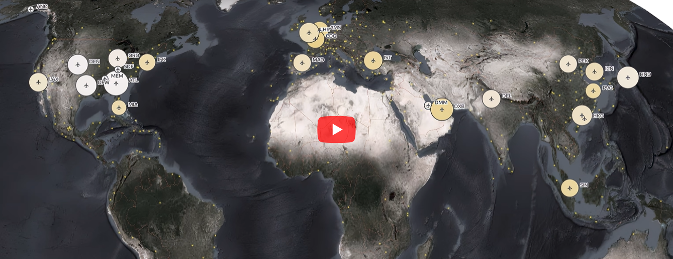
See examples and expressions in action in this video walkthrough.

Article Discussion: