Step‑by‑Step Guide: Local Relief Mapping with Raster Functions

World Local Relief Service Retiring

The ArcGIS Online-hosted image service World Local Relief, first published nearly ten years ago, will be retired in December 2026. This blog shows how to build your own local-relief raster anywhere in the world using Living Atlas elevation and ArcGIS Pro. You’ll decide the scale (neighborhood size), compute relief, and package a result you can reuse and share.

What is Local Relief?

Local relief is the elevation range – the highest minus the lowest point – within a chosen area (for example, within a 6 km neighborhood). It’s helpful because it shows how much the terrain varies within a local area—something a single elevation or slope value can’t capture—making it easier to understand the overall shape and complexity of the landscape. Applications of local relief include:

• Agriculture: Areas with steep local relief are often harder to farm due to equipment limitations and increased erosion risk.
• Urban planning: Local relief influences where roads can be built, how water drains, and where hazards like landslides may occur.
• Tourism and recreation: Activities such as hiking, skiing, and sightseeing are shaped by the presence and intensity of local relief.

Calculating Local Relief

We will use the World Elevation GMTED elevation dataset to calculate relief. This 250-m dataset was produced by the US Geological Survey (USGS) and National Geospatial-Intelligence Agency (NGA) in 2010.

We’ll focus on Portugal for this exercise. However, this workflow can be used for any area within the data export constraints of the elevation service. Downloading data is limited to a maximum area of 16,000 x 16,000 pixels, an area approximately the size of Europe.

Data Preparation

Download the ArcGIS Pro project package here. Double-click the downloaded file to open the Pro project that includes two data tables and the completed “Local Relief” Raster Function Template for verification of your work. Use this project for the steps below.

Step 1: Add elevation data to Pro

• Open the Add Data dialog box, search for “World Elevation GMTED” in the Living Atlas data source. Add the layer to your project.
• Repeat the Add Data steps, but this time, search Living Atlas for “country boundary generalized.” This feature layer will be used to isolate an area of interest—in this case, the country of Portugal.
• Your Contents pane should look something like this, with two Living Atlas layers added.

Step 2: Isolate an area of interest using country boundaries

• Change the symbology of the “World_Countries_Generalized” layer to Black Outline (1pt).
• Apply a Definition Query to this layer, set ‘Country Name = Portugal’.
• Right-click the layer and select “Zoom to Layer” to zoom into Portugal.

Step 3: Reproject elevation to ETRS 1989 Portugal TM06

We reproject the data so that distances and areas are accurately represented for Portugal, ensuring that the neighborhood used in later steps reflects true ground distance.

• Open the Project Raster geoprocessing tool.
• Fill in the tool parameters as shown below to reproject the area of interest to the local projected coordinate system for Portugal. Use the Memory Workspace as the output location.

• Turn off visibility for the “World Elevation GMTED” layer.

Step 4: Calculate the Range, Reclassify the output, and Symbolize the Results using Raster Functions

Step 4A: Calculating the range: We’ll use the focal statistics functions to calculate the range of elevation with a local (focal) window.

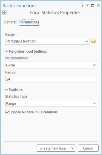
• Open the Raster Functions tool pane from the Imagery tab, search for and open the Focal Statistics function.
• Fill in the tool parameters as shown below and click ‘Create new layer’ to calculate the range using a circular neighborhood with a 6-kilometer radius. For our 250-meter resolution elevation raster, that equals 24 pixels.

• Right-click the result of the focal statistics function in Contents and select Edit Function Chain to open the editor pane.
• Search the Raster Functions pane for Remap. Drag the function onto the editor.
• Click the Focal Statistics function in the editor and drag the arrow over the Remap function and release it. This will connect the functions with a forward arrow.

Step 4B: Classify Local Relief Values for Visualization

The Focal Statistics tool in the previous step produced a continuous surface of local relief values, measured in meters. To make this surface easier to interpret visually, we’ll group the continuous values into broader relief categories using the Remap function.

This classification step simplifies the output—for example, by placing all values from 0 to 30 meters in one class, 30 to 60 in another, and so on. Grouping values in this way helps highlight major differences in terrain while minimizing distraction from small, insignificant changes (like one or two meters of variation).

• Double-click the Remap function to open the properties. Change the ‘Remap Definition Type’ to “Table”. Click the browse button on the ‘Remap Table’ field, navigate to the “Local Relief” file geodatabase, select the ‘Reclassify_Relief’ table, and click ‘OK’
• Complete the Remap Properties by making the following selections and clicking ‘OK’.

Parameters Tab

Input Field: From_Value

Output Field: New_Value

Input Max Field (optional): To_Value

General Tab

Output Pixel Type: 16 Bit Unsigned

Step 4C: Apply a Color Map for Visualization

Now that the relief values have been grouped into classes, we’ll assign colors to those classes to make the map easier to read and interpret. By connecting the Remap output to a color map using the Attribute Table function, we ensure that each relief class is displayed consistently and clearly using a predefined color scheme.

• Search for the Attribute Table function and drag it to the editor.
• Connect the Remap function to the Attribute Table function.
• On the Attribute Table function properties window, select “External” from ‘Table Type’ and select the “Color_Map” table from the “Local Relief” file geodatabase, click ‘OK’ twice to confirm. Your raster function template should look something like this.

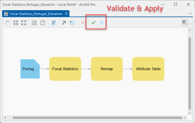
• ‘Validate’ the raster function chain, then ‘Apply’ the edits
• Close the Raster Function Editor to see the results

Using Raster Functions in this way results in a temporary in-memory local relief for the country of Portugal. To save this result, you can use the Copy Raster geoprocessing tool to output the result to a permanent raster file format such as TIFF.

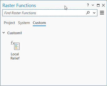
If you have any trouble building your own Raster Function Template (RFT), your Pro project includes a completed RFT called “Local Relief” under the Custom tab of the Raster Functions pane. You should be able to apply this RFT to your reprojected Portugal elevation data.

Now you have a repeatable workflow you can use to create your own local relief data for any place in the world. You can also save and share your RFT with colleagues.

Additional Resources

• Raster functions in ArcGIS Pro Documentation
• Raster function template properties in ArcGIS Pro Documentation

More Information

Join us at the Esri Community for expert advice, answers to your questions about Living Atlas, and much more!