Visualize and animate flow in MapView with a custom WebGL layer

Introduction

This article discusses visualizing wind and water currents through animated streamlines; the out-of-the-box capabilities of the ArcGIS API for JavaScript (ArcGIS JS API) are combined with custom WebGL code to create compelling animated visualizations of real-world atmospheric and marine data.

See it live or check out the source code on GitHub.

Custom layers are an advanced topic; familiarity with WebGL and custom WebGL layer views is recommended. A good place to get started with extending the ArcGIS JS API with custom WebGL layer views is the official SDK sample. And remember that your fellow developers at community.esri.com are always happy to help!

With that said… everyone deserves amazing maps! Streamlines are a natural drawing style for flow datasets, and our team is considering adding them to the ArcGIS JS API. Join the discussion on community.esri.com and share your ideas on how to bring this awesomeness to a larger audience!

The power of animations

Awesome datasets need awesome visualizations. The ArcGIS JS API ships with 2D and 3D support and a variety of layer types, renderers, effects, and blend modes that should cover the requirements of most users most of the time.

In this blog post, we focus on animated visualizations; animations can capture and communicate the dynamicity of certain datasets more effectively than static graphics. The ArcGIS JS API supports several forms of animations out-of-the-box and my colleague Anne Fitz penned down a great writeup covering several useful techniques that are applicable in a broad range of situations. With that said, certain applications call for a more customized experience; this is where custom WebGL layers come into play.

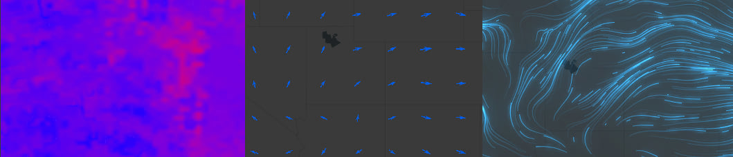
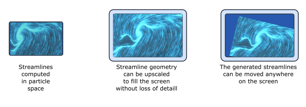
The images below show the same area of the map rendered in three different ways. For this article, we are focusing on an imagery tile layer containing wind magnitude and direction for the continental United States.

• Predefined ImageryTileLayer with "raster-stretch" renderer (left). This option does a good job at visualizing wind speed, but the direction information is lost.
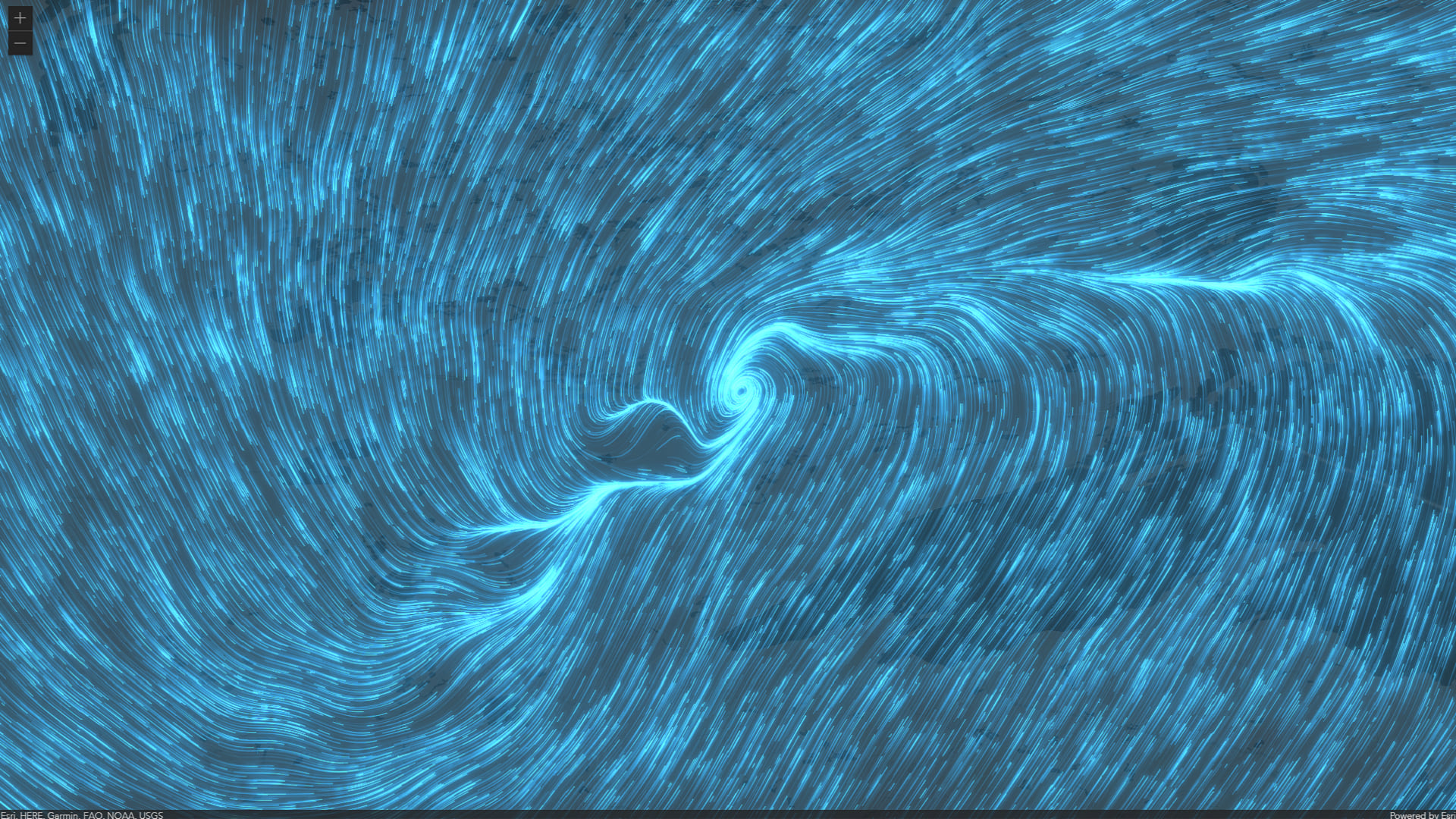
• Predefined ImageryTileLayer with "vector-field" renderer (center). Using arrow symbols and size and rotation visual variables, this renderer can visualize both aspects of the wind. ImageryTileLayer support for this renderer is shipping with version 4.21 of the ArcGIS JS API; before that, this new functionality is available in the next build.
• Custom WebGL layer displaying animated flow lines, as described in this article (right). Our custom visualization provides a more intuitive representation of wind currents; the different animation speed of the lines maps to the underlying concept of speed magnitude, and the continuous nature of the visualization makes it easier to spot patterns in the data, like that rotational flow near the Canadian border. Also, it looks pretty cool.

This article describes in depth the implementation of a custom WebGL layer that displays animated streamlines. A streamline is the path that a massless particle would take when immersed in the fluid. Please note that the focus of the article is on the flow visualization algorithm and integration with the ArcGIS JS API; whether the particular technique is suitable for a given dataset, audience, or application, needs to be evaluated by a domain expert, and the implementation modified as needed.

Load, transform and render

As anything that shows up on a computer screen, GIS visualizations are the result of:

1. Loading the data;
2. Optionally, transforming/processing/preparing the data;
3. Rendering the data!

Each of the predefined layer types that ship with the ArcGIS JS API is a software component that bundles together two capabilities.

• The ability to access data, either from local memory or from a remote source;
• The ability to render the retrieved data, often both in 2D MapView and 3D SceneView.

In the ArcGIS JS API, the implementation of a layer type consists of a layer class and one or two layer view classes. With relation to the three phases discussed above, the layer is mostly responsible for accessing the data (1) while 2D layer views and 3D layer views take care of the rendering (3). Data transformation (2) can be required for different reasons and, to some degree, it is carried out both by layers and layer views.

Polylines with timestamps

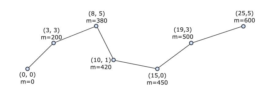
At the core of a visualization such as the one that we are setting out to build, there is the concept of a m-aware polyline feature. This is a polyline where each vertex, in addition to its coordinates, carries one or more m-values. An m-value can be thought of as a position dependent attribute of the polyline, that varies smoothly along its path; for vertices the m-value is given explicitly, while for any points between two vertices it can be obtained by linearly interpolating the value at the vertices.

A common application of m-aware polylines is representing paths or, as in this article, streamlines; in this case the m-values are the timestamps at which that vertex is visited by the particle.

If your data is already stored in an m-aware polyline feature layer, FeatureLayer.queryFeatures() can be used to retrieve the polylines and access the m-value information.

Catching wind

In this article we will not ingest polyline features; we will build the polylines starting from flow data contained in an ImageryTileLayer. This layer type is similar to ImageryLayer in the sense that it contains raster LERC2D data, but the way that the data is stored on the server is different; imagery tile layers store data into static files called tiles, that are cloud and cache-friendly. Each tile contains many pixels, and each pixel contains one or many bands of data. In the case of an imagery tile layer that stores wind data, there are two bands that together describe wind direction and speed.

As it is the case with any other predefined layer, an ImageryTileLayer can be added to a map and displayed by a MapView. The simplest way to visualize an imagery tile layer is with a "raster-stretch" renderer. The default settings are usually sensible, and the resulting visuals are easy to interpret with the help of a legend. See the "raster-stretch" renderer in CodePen.

We will focus our attention on imagery tile layers that store flow information, such as wind and marine currents. For these kind of layers, the "vector-field" renderer is supported and used as the default renderer. See the "raster-stretch" renderer in CodePen.

Watch this space!

The input to a rendering algorithm is visual in nature, or at the very least can be interpreted as visual. For instance, positions are expressed as numbers and the rendering algorithm is responsible for drawing geographic entities in the right places according to those numbers. However, numbers by themselves are meaningless, and they only get their positional semantics from being associated to particular spaces.

In the course of this article we are going to refer to three spaces; each space plays its own role in the implementation of the streamlines visualization.

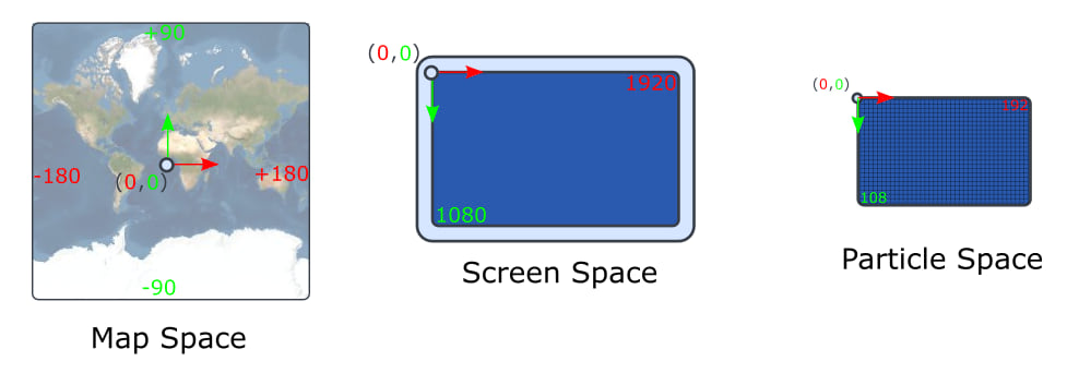
Map space

Map space is used to locate the data on the server. In the case of the wind imagery tile layer that we are considering in this article, it is given by the EPSG:4326 reference system. Map space is right-handed and its coordinates are expressed in map units.

Screen space

Screen space is the left handed frame where +X is right, +Y is down, the origin is in the upper-left corner of the MapView, while the lower-right corner has for coordinates the width and height of the MapView. Screen space coordinates are expressed in pixels.

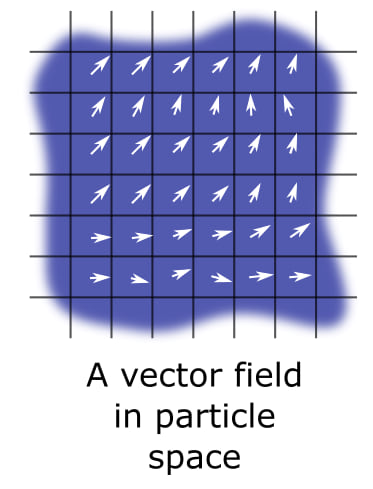
Particle space (aka model space, aka object space aka local space)

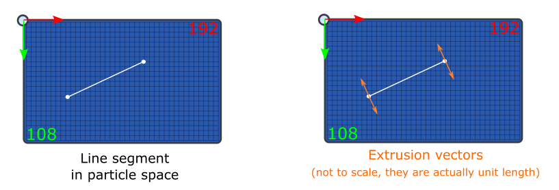
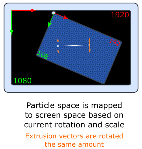
The animated lines are the result of a particle simulation. The position of a particle as it is swept by the simulated wind traces the polyline that will be later animated. The position of a particle is expressed in particle space. The units of the particle space are called cells and are related to pixels by a multiplicative constant, called cellSize. In the figure above we assume cellSize of 10 so that a 1920x1080 pixels MapView results in a 192x108 particle space.

We will see that streamlines ultimately will be rendered using triangle meshes; the coordinates of mesh vertices will be expressed in particle space; in computer graphic, this space is often called model space, object space, or sometimes even local space.

Vector fields

A field is a position-dependent property of a space. Temperature, pressure, humidity are all examples of scalar fields common in meteorology. In other words, a scalar field maps a point to a numeric value. In GIS systems scalar fields are often represented using one band of an imagery tile layer.

Some properties are multidimensional in nature, and they are called vector fields. This article focuses on a specific type of vector field, useful to represent wind data, called a velocity field; a velocity field associates a velocity vector to each point of a space. A velocity is a “directional speed” and can be represented using two bands of an imagery tile layer. There are two different ways to encode 2D velocities.

Magnitude and direction

This is reported as “dataType”: “esriImageServiceDataTypeVector-MagDir” in the raster info section of the layer.

The direction of the wind is measured in degrees, with 0 being North and 90 being East. The magnitude is a speed.

UV

This is reported as “dataType”: “esriImageServiceDataTypeVector-UV” in the raster info section of the layer.

U is a the west-east component of the speed and V is the south-north component.

Fetching the LERC2D wind data

In the ArcGIS JS API, layers do not have to be added to a map to be useful; several layer types offer data fetching capabilities.

This is especially remarkable for ImageryTileLayer.fetchPixels(), which enables querying arbitrary extents in spite of the fact that the queried data is broken into tiles on the CDN. The implementation of ImageryTileLayer takes care of downloading the (possibly cached) tiles and stitches them together in a single image that spans the required extent.

An instance of ImageryTileLayer can be used to fetch the data that a custom WebGL layer view needs. Every time that the MapView becomes stationary, the custom WebGL layer view triggers a refresh of the visualization. The current extent of the visualization is passed to ImageryTileLayer.fetchPixels() together with the size of the desired output LERC2D image. Instead of querying an image of the same size of the MapView, we ask for a downsampled image by a factor of cellSize, which is fixed at 5 in the current implementation. As an example, if the MapView was 1280×720, the code would fetch a 256×144 image from the image server. We do this to save bandwidth, reduce processing time, and “regularize” the data; full-resolution wind data may have high-frequency components that are likely to destabilize the simulator. The downsampled image represents the wind in particle space and each data element is called a cell.

The rawCellData stores the two bands of the wind separately, in two distinct, row-major, equally sized matrices. Whether these two bands are MagDir or UV can be determined by examining the rasterInfo.dataType property. We chose to normalize the values to particle space UV, which is more convenient for the simulation, and interleave the two bands into a single matrix. Note that the original values would have probably been expressed in knots or meters per second, but from now on we will assume that all velocities are in particle space.

There are a couple of things worth mentioning about the conversion formulas.

In the “MagDir to UV case” the magnitude is multiplied by sine and cosine factors to get the U and V components respectively. Note how the direction is first converted to radians, and then it is delayed by Math.PI / 2; this is needed because in particle space positive angles rotate the +X axis over the +Y axis, while in map space positive angles rotate the +Y axis (the “North”) over the +X axis (the “East”). These two conventions are both clockwise but angles in map space are a quarter of a full circle late.

In the “UV to UV case”, the U value can be copied but the V value needs to be flipped, because in particle space +Y goes down while in map space it goes up.

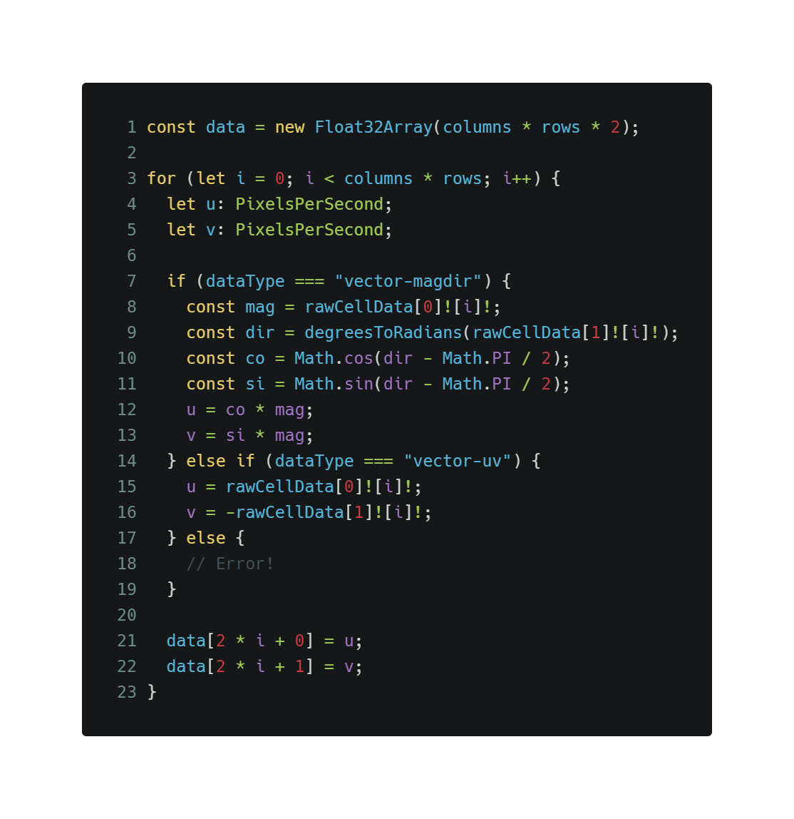
The output of the fragment of code above is the data variable that essentially is a discretized velocity field in particle space; i.e., each cell in particle space is mapped to a horizontal velocity (+X is right) and a vertical velocity (+Y is down), also in particle space.

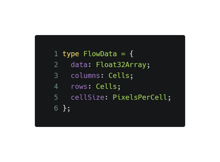
In the rest of the article, FlowData denotes a type that holds the data variable, together with the grid dimensions and the cellSize factor. FlowData is the input to the particle simulation code that traces the streamlines in particle space.

Pro tip: smooth the data

We already “smoothed” the flow data by requesting the image server a lower resolution image than the MapView itself. In addition to this, for certain datasets an explicit smoothing using a separable Gaussian kernel can help obtaining more robust and aesthetically pleasing results.

Turning the particle space vector velocity field into a function

For ease of use by the particle simulator, we wrap the flowData.data typed array into a closure; the closure takes a point (x, y) in particle space and returns a velocity again in particle space.

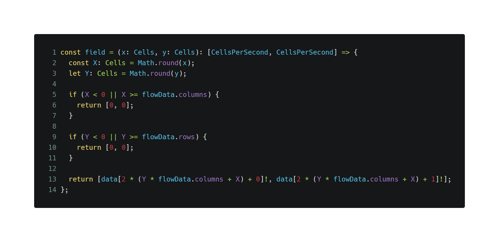
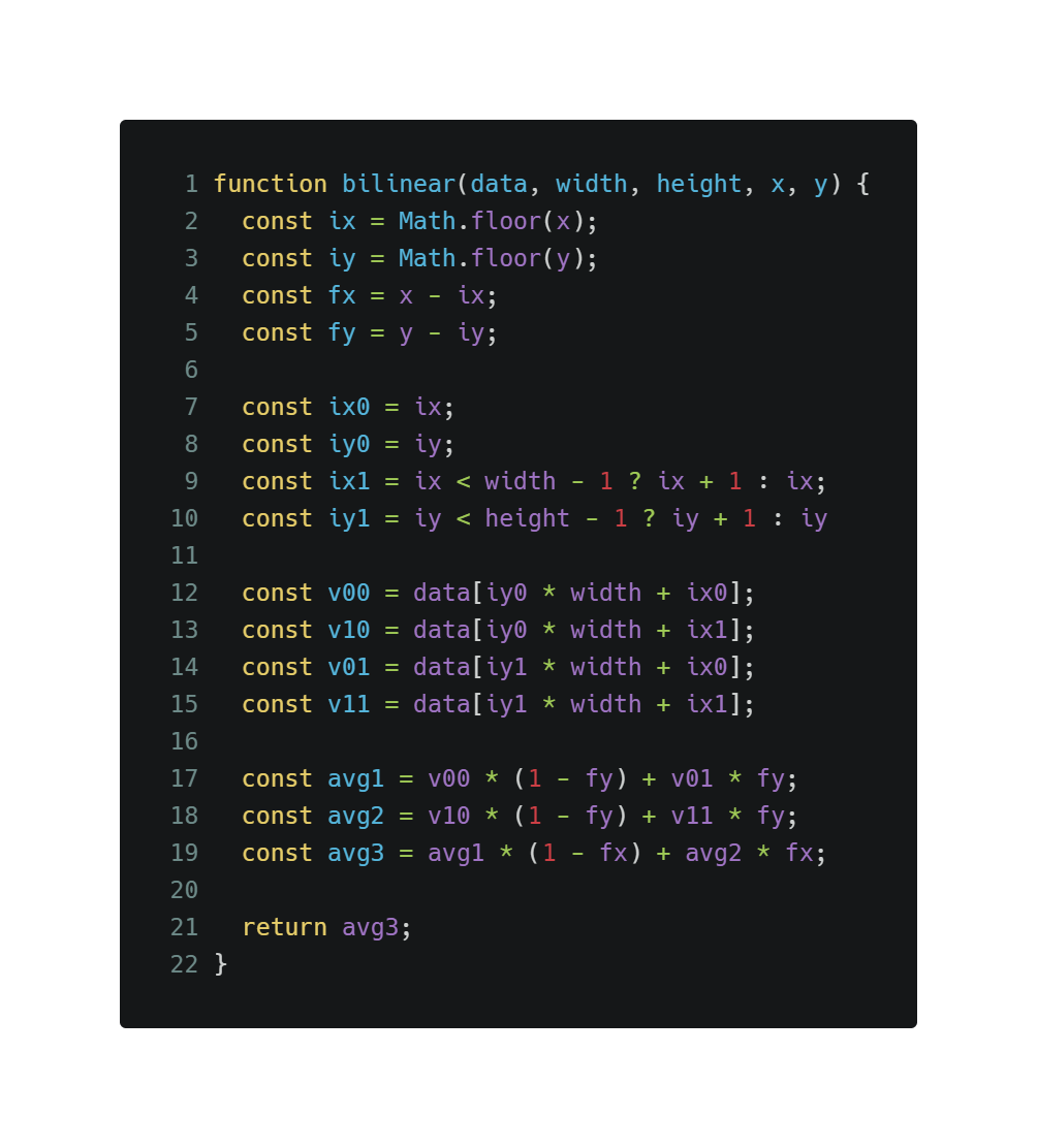
Pro tip: adopt bilinear interpolation

A simulated particle will have more often than not a fractional position, i.e. (42.23, 89.54). With such input, the field closure defined above would take the velocity in cell (43, 90) and return that. A better way of coming up with a value for fractional positions is to use bilinear interpolation; this allows for the velocity field to vary smoothly across a single cell and could be required to get acceptable results from the particle simulation when the wind data is low resolution.

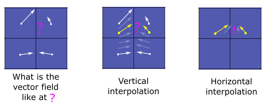
Bilinear interpolation works by selecting the four closest cells; first two adjacent pairs of cells are interpolated vertically, based on the distance of the desired point from the cells’ centers, and then the results of the first interpolation are interpolated again horizontally. See bilinear interpolation for more details.

Particle simulation

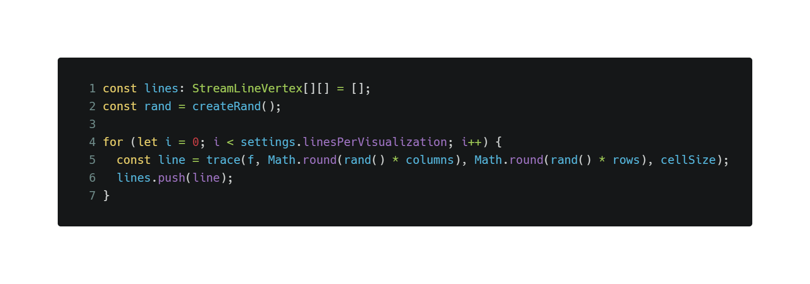
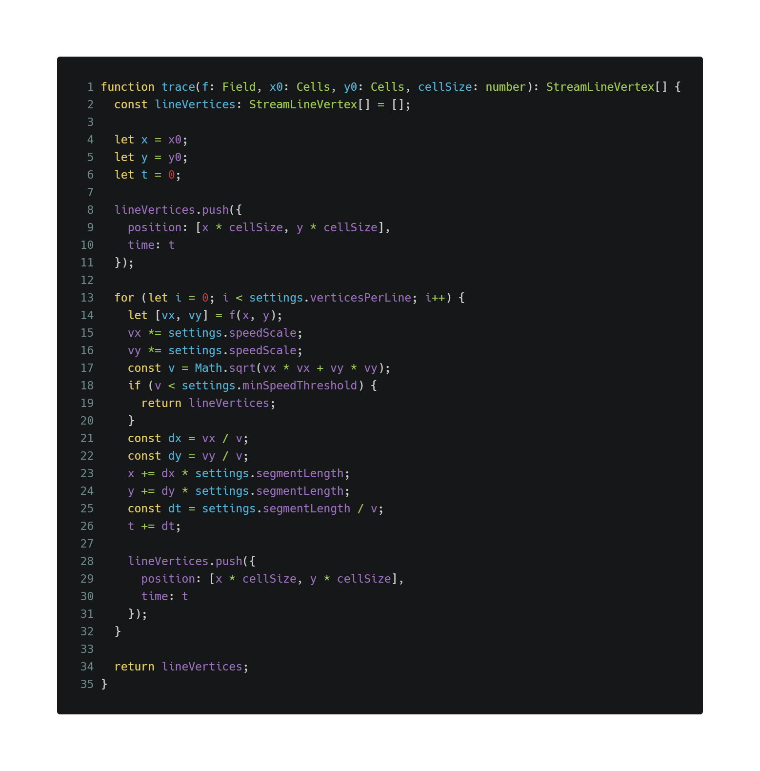
Particles are immersed in the closure-wrapped FlowData field at a pseudo-random (but repeatable, using a seeded generator) positions and simulated using the trace() function.

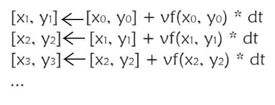
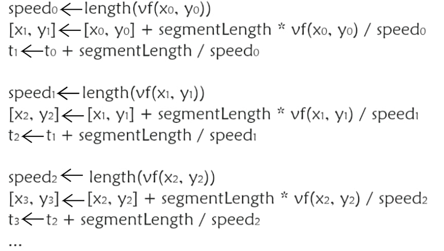
Simulating the movement of a particle in a velocity field vf is an iterative process, for which there are a couple of different approaches. The simplest one uses a fixed time step and increments the position of the particle by an amount proportional to the velocity at that point and the time step. Each iteration produces a new vertex of the polyline and, together with the previous vertex, a new segment.

Fixing the time step is a perfectly sound approach but for the demo app we opted for a fixed segment length instead. This approach causes line lengths to vary less and also guarantees that adjacent vertices are not too close to each other; we think that both these properties are desirable for this kind of visualization, but the reader is encouraged to experiment with different iteration strategies.

In the demo app, each particle is update 30 times using a for loop and the segment length is 1 cell; together with a cellSize of 5 pixels, this leads to each individual polyline having a length of about 150 pixels. At each iteration the speed of the particle is tested and, if found to be too low (because the particle entered a cell where the wind is weak), the simulation for that particle is terminated.

Building the triangle mesh

WebGL has poor built-in support for line drawing; all the line rendering capabilities that ship the ArcGIS JS API are based on triangle meshes, and for this custom flow WebGL we are taking a similar approach. For more information, check out the SDK sample about animated lines. Also, the reader should be aware that the ArcGIS JS API ships with tessellation helper methods that can convert arbitrary geometries into triangle meshes.

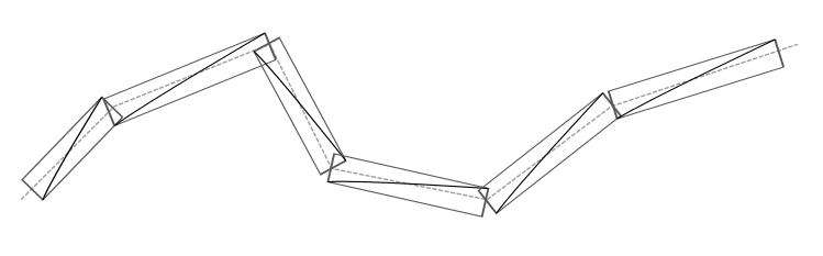
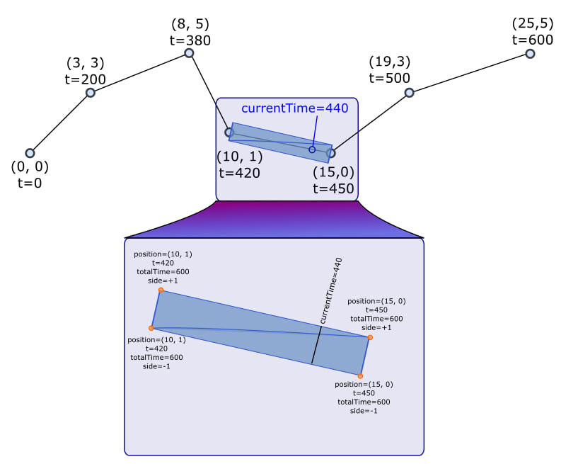
For representing streamlines our visual requirements are quite basic and we are going to stick with a very simple method; each segment of a polyline is represented by a thin rectangle, at most 2-3 pixels wide, lying along the original polyline; the original polyline becomes the centerline of this “rectangle chain”. Each rectangle is made of 4 vertices, 6 indices, and renders as a pair of right gl.TRIANGLES sharing their hypothenuse. This approach leads to gaps and regions of overlaps, but it is a very fast and robust algorithm, and for thin lines, the artifacts are not noticeable.

In the next paragraphs, we call polyline vertex a vertex of the original polyline, as produced by the particle simulation algorithm. Such vertex is extruded in directions perpendicular to the centerline to produce mesh vertices; these are the vertices that are written to the WebGL vertex buffer.

The most powerful feature of low-level, GPU-accelerated graphic APIs like WebGL, that really sets them apart from Canvas2D, GDI+ and all the other higher-level solutions, is the ability to define custom visual properties, and use them in custom programs called shaders. This enables applications to describe complex scenes, with many different, possibly animated, objects, and render them with little assistance from the CPU. This approach greatly reduces the load on the CPU, and the GPU is free to run at full speed.

There are going to be about a thousand streamlines in a typical flow visualization; we want to render all of them using a single draw call. To achieve this, we need to store all triangle meshes for all polylines in the same vertex and index buffers. The code snippet below does just that. Note that since this could be a long-running process, the algorithm is designed to transfer control back to the event loop once in a while so that the UI thread does not freeze (lines 12-15).

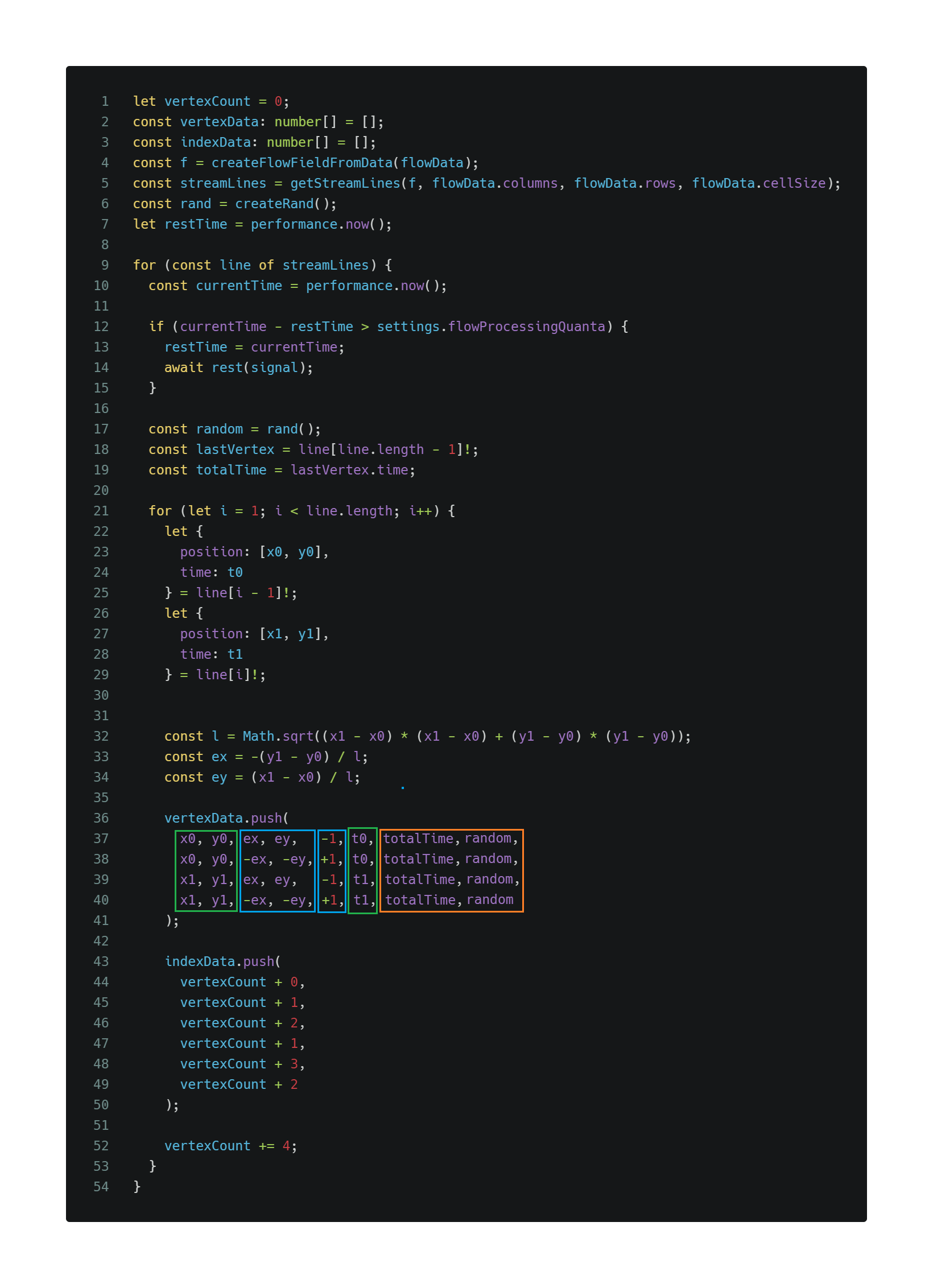
The custom properties that we need to define fall into 4 categories.

Per-frame
These properties are shared by all polylines and are updated every frame. They are passed to the shaders using uniform values. Since they do not need to be stored in the vertex buffer, we will talk about them when discussing rendering.

Per-feature
These properties are associated with the polyline itself. The only way to implement this kind of property in WebGL 1, while at the same time maintaining the ability to draw all polylines with a single draw call, is to actually make them vertex attributes, and repeat the same values for all vertices of the same feature.

There are 2 per-feature properties:

– totalTime is the total runtime in seconds for the polyline. The fragment shader needs this value at every fragment in order to properly loop the animation.
– random is a pseudo-random value, again needed in the fragment shader to introduce some temporal differences in the animation, so that streamlines with the same length do not end up synchronized.

They are highlighted in orange in the code snippet above.

Per-polyline-vertex
These properties are associated with the polyline vertex itself. There are 2 per-polyline-vertex properties:

– x, y, the vertex position, in particle space units, i.e., cells.
– t, the vertex timestamp.

They are marked in green in the code snippet.

Per-mesh-vertex

Each polyline vertex is extruded into two mesh vertices, one per side of the polyline. There are 2 per-mesh-vertex properties.

– ex, ey is the extrusion vector. This is computed at lines 32-34 by normalizing the segment vector and rotating it 90 degrees. Being normalized, its magnitude is meaningless but you can imagine it being expressed in particle space units, i.e., cells.
– a +1/-1 constant that we call side, and identifies an extruded vertex as lying on the right side of the centerline, or on the left side.

They are marked in blue in the code snippet.

For more information about constructing and rendering line meshes, see the SDK sample about animated lines.

Rendering

Now is time to put the GPU to work and render our beautiful streamlines!

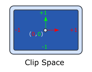
Before discussing rendering there is one additional space that needs to be introduced; it is called clip space and just like screen space describes positions on the screen, but using a different coordinate system. In clip space, the origin is in the center and the drawing area is seen as a 2x2 rectangle, where +X is right and +Y is up. This space is the space of the gl_Position variable.

The rendering process takes the particle space mesh and draws it to the screen. As the user pans and zooms, the visualization needs to be repositioned to reflect the change in view point, until a new mesh is ready that again can be rendered full screen.

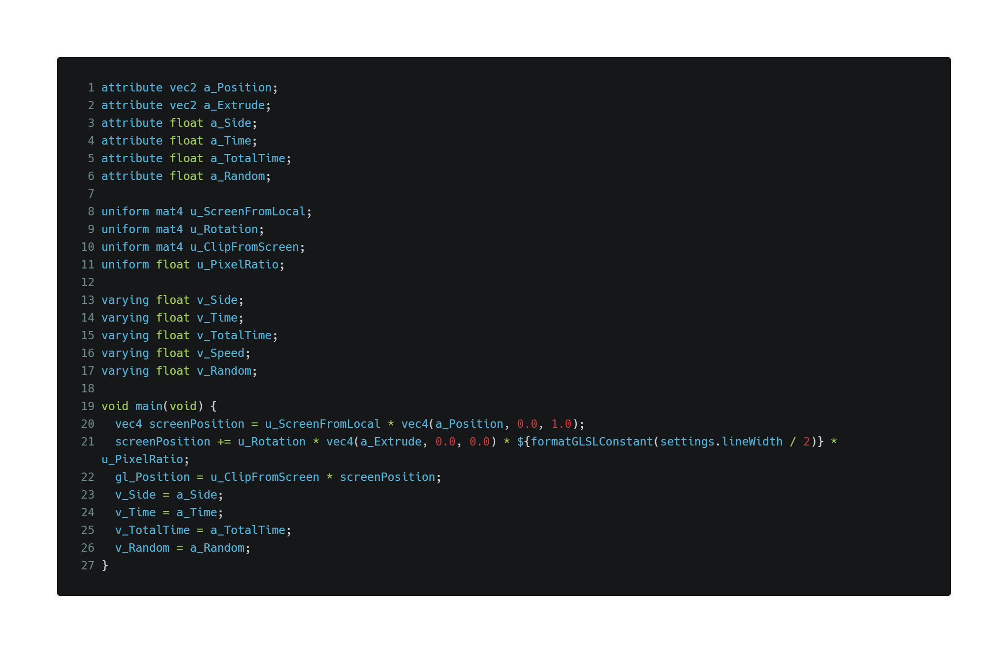
Vertex shader

The vertex shader converts the coordinates of mesh vertices from particle space to screen space using the u_ScreenFromLocal matrix, extrudes them according to the extrusion vector, and then transforms everything to clip space using the u_ClipFromScreen matrix. Note how the extrusion vectors are rotated by the u_Rotation matrix and scaled by half line width but are not subject to the same transformation that particle space coordinates go through, which also includes a scale factor when zooming in and out; this separation between position and extrusion vectors is responsible for the anti-zoom behavior of lines, which always exhibit the same width. The value u_PixelRatio is used to display lines always of the desired width, even when the DPI of the screen is very high or very low.

All other attributes are passed verbatim to the fragment shader using varying variables.

Fragment shader

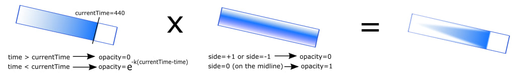
The fragment shader creates and animates the trail effect.

It does so by taking advantage that each fragment is associated with a timestamp, computed automatically by the GPU interpolator based on the timestamps at the two closest vertices.

The next snippet shows the fragment shader source.

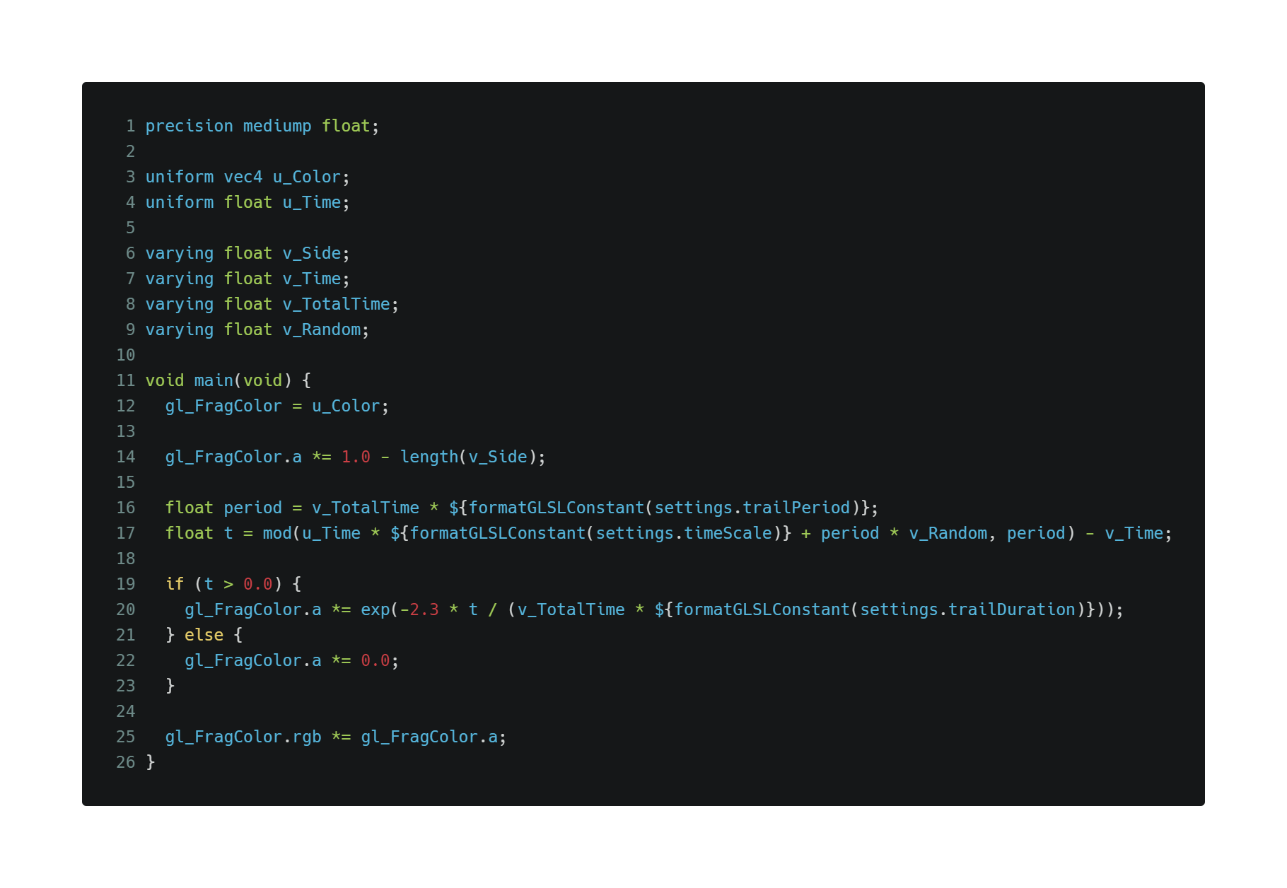
The base color of the streamlines is taken from uniform u_Color. The fragment shader modifies the opacity of the fragments to implement the animated trail effect.

A fragment tends to be opaque when its timestamp is close but not greater than the current time, which is passed to the shader as the uniform u_Time; this is done at lines 16-23 using an exponential function applied to a periodized time-dependent signal.

A fragment is also more opaque on the centerline than near the edges of the rectangle; this effect is applied at line 14 by taking advantage of the fact that the a_Side attribute has an absolute value of 1 near the edges, and 0 on the centerline.

Finally, at line 25 the output color is premultiplied because MapView will not composite the layer correctly otherwise.

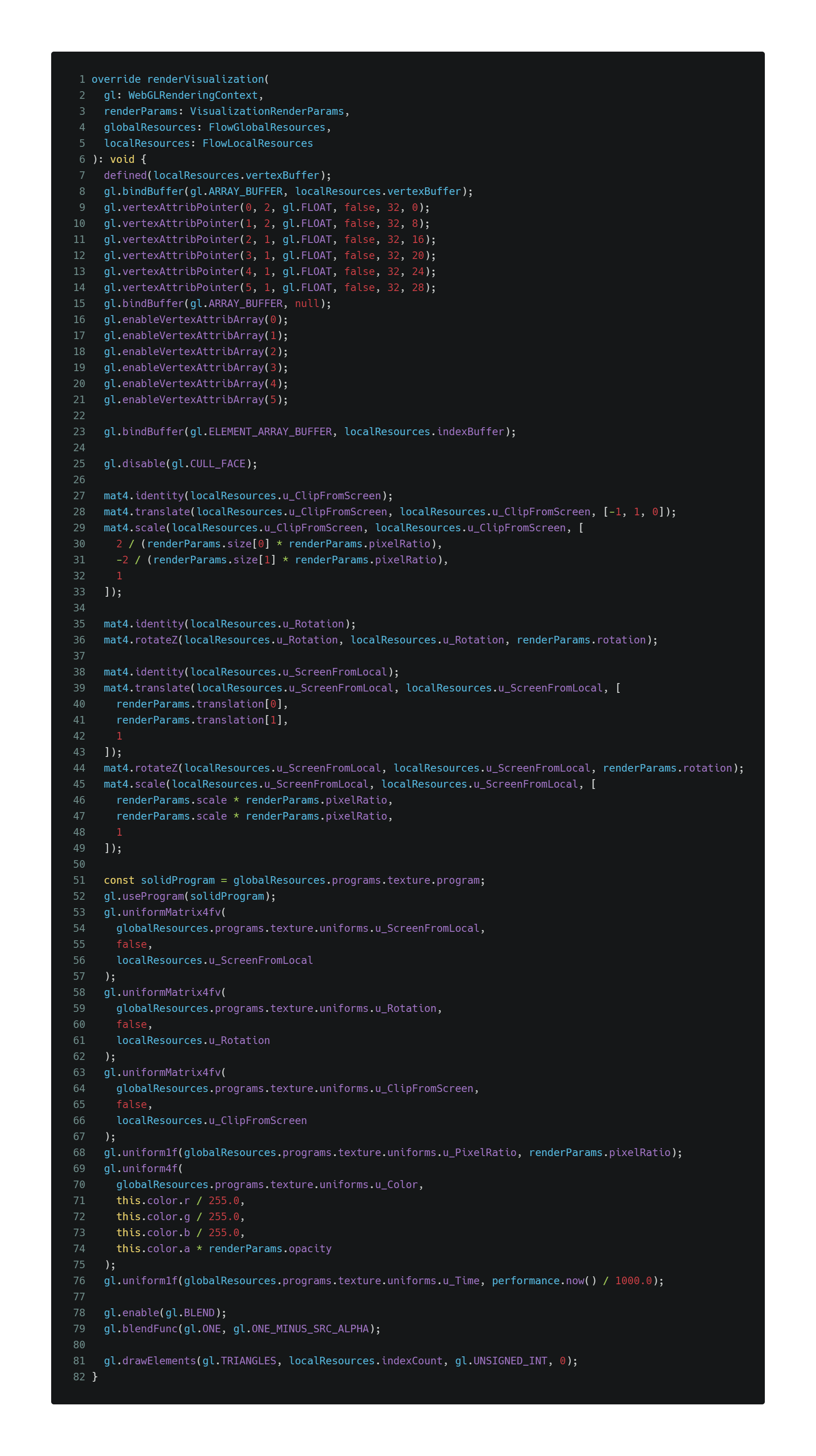
Configuring WebGL and issuing the draw call

We are ready for rendering! The rendering algorithm consists of about 80 lines of WebGL state setting and a single draw call.

– Bind the mesh (lines 7-23)
– Build the u_ClipFromScreen matrix, that transforms from screen space to clip space (lines 27-33).
– Build the u_ScreenFromLocal matrix, that transforms from particle space to screen space (lines 38-49).
– Build the u_Rotation matrix, used to rotate extrusion vectors (lines 35-36).
– Configure the shader program (lines 51-76).
– Enable premultiplied alpha (lines 78-79).
– Draw all the streamlines at once (line 81).

Putting everything together

In the source repository the code is chiefly organized around two packages; core and flow.

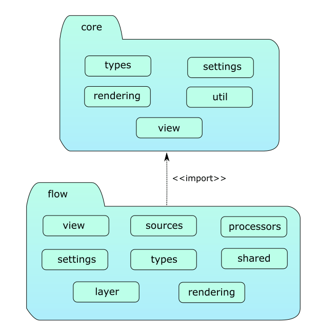
core
The core package contains generic classes and utilities that are useful to create custom visualizations; it provides a simpler abstraction on top of BaseLayerViewGL2D and implements the resource loading/unloading lifecycle. It contains the following modules.

– types. Type definitions and interfaces used by the entire codebase. Most importantly, it introduces the concept of global resources and local resources. Global resources are loaded at startup and do not need to be updated when the extent changes; local resources are tied to a particular extent and needs to destroyed and reloaded as the user navigates the map.
– settings. Constants that define some of the built-in behaviors of the flow package; in a real-world app these should probably be configurable at runtime.
– util. Functions of general utility.
– rendering. Defines the abstract class VisualizationStyle, a class that defines how to load global resources, how to load local resources for a given extent, and how to render a visualization. It is an abstraction over the attach()/render()/detach() contract offered by BaseLayerViewGL2D and its concrete implementations can be ran and tested without a running MapView. You can even create a static image out of a visualization style, for instance to be used as a thumbnail, by calling method VisualizationStyle.createImage().
– view. Defines the abstract class VisualizationLayerView2D, a subclass of BaseLayerViewGL2D. It offers a simplified programming model and resource management scheme designed around the concept of visualizations, which are basically graphic objects that cover the current extent. To implement a new custom layer, inherit from VisualizationLayerView2D and override method createVisualizationStyle(). If the custom visualization is animated, set the animate flag to true.

flow
The flow package depends on core and implements the streamline rendering logic.

With relation to the architecture of a geographic visualization app, the flow package provides an implementation for each of the 3 required steps.

1. Loading the data;
2. Transforming/processing/preparing the data;
3. Rendering the data.

The flow package contains the following modules.

– types. Type definitions and interfaces used by the flow package.
– settings. Constants that define some of the built-in behaviors of the flow package; in a real-world app these should probably be configurable at runtime.
– sources. Defines different strategies for loading (1) flow data; two strategies are supported at present time: ImageryTileLayerFlowSource that fetches LERC2D datasets from an imagery tile layer, and VectorFieldFlowSource that supports the analytic definition of a global velocity field in map units.
– processors. Defines the entire data transformation (2) pipeline, starting from flow data, particle simulation, conversion to streamlines and generation of the triangle mesh. Class MainFlowProcessor uses the main process, while WorkerFlowProcessor uses the workers framework.
– shared. Particle simulation and mesh generation code that can be invoked both by the main process, when useWebWorkers is false, and by the worker when it is true.
– layer. Defines the FlowLayer class by inheriting it from esri/layers/Layer. This class overrides method createLayerView() to return an instance of FlowLayerView2D.
– rendering. Defines three classes: FlowGlobalResources, FlowLocalResources and FlowVisualizationStyle. These are concrete implementations of the abstract concepts defined in the same name module in the core package.
– view. Defines the FlowLayerView2D class by inheriting it from VisualizationLayerView2D. This class overrides method createVisualizationStyle() to return an instance of FlowVisualizationStyle.

The codebase contains a couple more interesting things that we have not been able to cover in this blog post, due to space constraints; first, FlowLayer defines a way to specify client-side flow data, which can be very useful for education and what-if scenarios where real data is not available.

Finally, FlowLayer supports running the particle simulation and mesh generation on workers, to reduce the load on the main thread that could lead to possible UI freezes. Workers are enabled by default and are controlled by the useWebWorkers flag.

The main application file

The main application file declares a VectorTileLayer to be used as a basemap, an ImageryTileLayer that will be displayed by the standard vector field renderer, and our brand-new FlowLayer pointed to the same imagery tile layer URL.

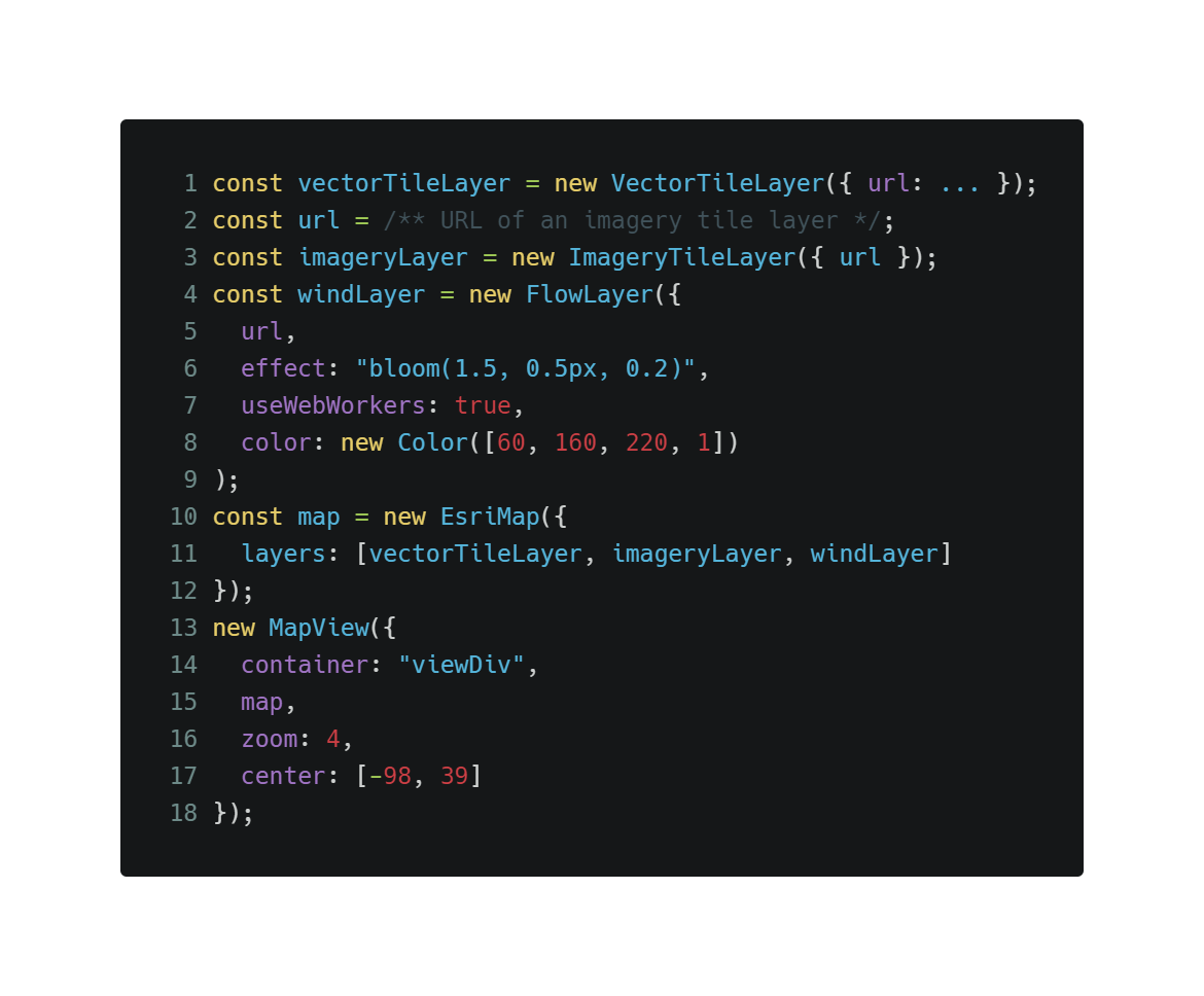
And… we are done!

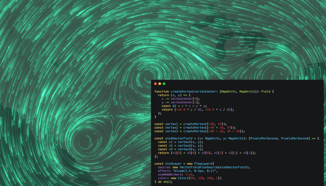
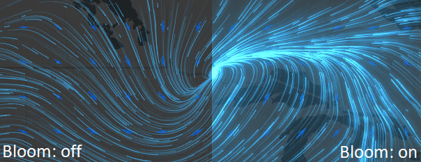
It is quite remarkable that a bunch of blue rectangles and less than 60 lines of shading code can look so pretty. The secret is that there is more shading going on behind the scenes; the FlowLayer that we just created is compatible with blend modes and layer effects. A large share of the visual appeal comes from specifying effect: "bloom(1.5, 0.5px, 0.2)" when creating the FlowLayer instance.

The image below shows the positive influence of the bloom effect on our custom visualization. We encourage you to try other effects and blend modes, as well as stacking other predefined operational layers on top or below FlowLayer.

Conclusion

We hope you enjoyed this deep dive into flow visualization and animation using the ArcGIS JS API and custom WebGL layers. Check out the source repository and try to modify FlowVisualizationStyle to create your own dream layer.

On behalf of the ArcGIS JS API team, we thank you for your interest in flow visualization; we are thinking that this drawing style is important enough that it should be a native capability of the ArcGIS JS API. We would love for you to join the discussion on community.esri.com and share your use case, workflow, or requirements with us.

Happy coding!