By Rajinder Nagi, Esri Research Cartographer
We are pleased to announce the release of the new ArcGIS Bump Map Tools! This new toolbox contains tools to help you create and symbolize “bump maps” which are used by cartographers to add texture to a hillshaded surface. This technique is most often used to give the illusion of a realistic vegetated surface, though Jeff Nighbert has also talked in some of his papers and presentations about using it to represent rocky outcrops and other surfaces as well. Jeff introduced the technique to ArcInfo users at the 2003 Esri User Conference.
Bump mapping is done by first creating a random point pattern, using that pattern to create bumps as a raster surface, adding the bumped surface to the underlying DEM, hillshading the DEM, and then symbolizing the results.
Symbolizing the results includes two steps – 1) symbolizing the hillshade, and 2) symbolizing the vegetation overlay with a layer tint or other color. We will talk about this on our next blog post, Symbolizing the bump map.
The bump map model that Esri developed creates an output raster that represents the combination of multiple “bumped” surfaces, each relating to a different type of vegetation. It allows users to specify the parameters for each type of vegetation, including cones (for coniferous vegetation) or domes (for deciduous vegetation), as well as vegetation density (spacing), radius, and height. The model was built using two scripts that were written in the open source Python scripting language so they can be modified with ease. You can use other outputs from the model to symbolize the bumped areas that were created by the model. In addition, we build a No Bumps script that you can use to symbolize the areas where there are no bumps in the texturized surface. We will talk more about symbolizing the bump map in our next blog entry.
With these resources, you can easily and quickly create and symbolize data that gives a more realistic impression of hillshaded vegetated surfaces.
Let’s look the Bump Map model in a little more detail.
How the model is structured
The model was built using two scripts “Bump Map Script – Part 1” and “Bump Map Script – Part 2”, where Part 1 creates the random point pattern(s) based on user defined inputs about how the bumps for the vegetation should appear, and Part 2 creates the bumps (figure 1). Each vegetation type is represented by “bumps” that are defined by type (cones for coniferous vegetation or domes for deciduous vegetation), density (spacing), radius, and height. The vegetation pattern or patterns are then added to the DEM and hillshaded to create the final output. If necessary, the DEM is resampled, so the smaller the “bumps” (i.e., the user-defined radius), the longer the DEM will take to resample.
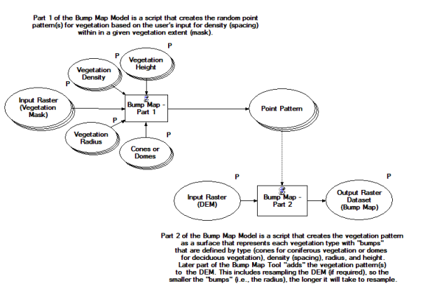
Figure 1. The structure of the Bump Map model.
Users should not run the scripts (Parts 1 and 2) individually as these are embedded in the Bump Map Model for seamless functionality.
Using the Bump Map model
First unzip the Bump Map Tools you can download from here. Take a moment to review the contents of the file once you unzip it. You will see the following (figure 2):
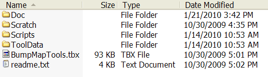
Figure 2. The contents of the download
Take a minute to read the readme.txt file for some detailed information on the contents of the download. Note that there is a ToolData directory and a Scratch directory. If you look in the ToolData directory, you will find some DEM and vegetation data that you can use to try out these tools. Intermediate data will be written to and deleted from the Scratch directory automatically when you run the tools.
One preparatory step is to make sure that the DEM and vegetation mask rasters you want to use are in the same coordinate system, and that they are projected so that the linear units are in either meters or feet.
Now you are ready to use the model. In ArcMap, right click in the ArcToolbox window and select “Add a Toolbox”. Navigate to the location of your download and select the BumpMapTools toolbox. Open the toolbox and double click the Bump Map Model. The user interface will look like figure 3:
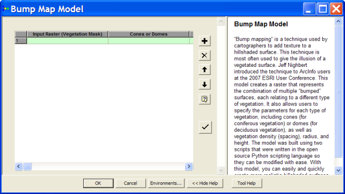
Figure 3. The user interface for the Bump Map model.
The input parameters include:
- Input Raster(s) (Vegetation Mask): The vegetation mask raster is a binary raster with the same value for cells in which the vegetation is present and NoData for all other cells. Here are two examples:
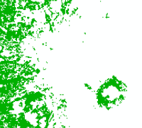 An input raster for vegetation that is only conifers.
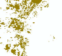 An input raster for vegetation that is only sedge.
- Cones or Domes: This is a drop down menu option where the user can select cones (to create a surface that represents coniferous vegetation) or domes (to create a surface that represents deciduous vegetation).
- Vegetation Density: This parameter will dictate how dense or sparse the cones/domes will be. Input a lower value to create a pattern that is denser and a higher value to create a pattern that is sparser. In essence, what happens is that a point will be placed randomly within each quadrilateral of an array that is defined by the value you input. If you input a value of 10, one point will be randomly placed within each quadrilateral of an array that is comprised of quadrilaterals that are 10 units by 10 units in size. The units for the value that you input to define the size of the quadrilaterals in the array is derived from the coordinate system for the input vegetation mask raster (usually either meters or feet).
- Vegetation Radius: Input a value that relates to how wide you want the bumps to appear. The value is the radius of each bump. The unit for the value that you input is derived from the coordinate system for the input vegetation mask raster. This value could have an impact on the amount of time it takes for this tool to run. If you input multiple vegetation masks, the LOWEST value for this parameter will be used to dictate the resampling for the DEM, if necessary, to which the bumps will be added. The new cell size will be the lowest radius value divided by 11 so that the bumps will appears to be nice and smooth. This means that if you input a 10 meter DEM and set a radius of 10, the output cell size for the final bump map and all the vegetation bump rasters will be less than one meter (i.e., 10/11).
- Vegetation Height (optional): Input a value that relates to how high you want the bumps to appear. This is a required value for creating cones, but not for domes. The unit for the value that you input is derived from the coordinate system for the input vegetation mask raster.
- Input Raster (DEM): This is the input DEM (not the hillshade!)
- Output Raster (Bump Map): This is the output raster that includes bumps for all the vegetation classes as well as the hillshade for the underlying DEM.
The model was developed to work in batch mode so that you can input parameters for multiple vegetation types. As with any other ArcGIS geoprocessing tool that runs in batch mode, each row represents a process and within each row, each cell represents one of the tool’s parameter (figure 4).
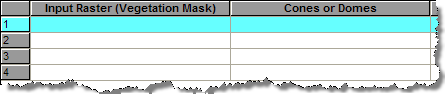
Figure 4. Typical interface for batch mode processing
Tip: Before running the model, please make sure the DEM and vegetation mask raster’s are in the same coordinate system and are projected so that the linear units are in either meters or feet.
Model output
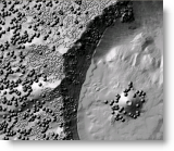
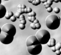
This model creates a hillshaded raster that represents the combination of multiple “bumped” surfaces atop with the underlying DEM, where each type of bumped surface relates to a different type of vegetation, as shown in figure 5.
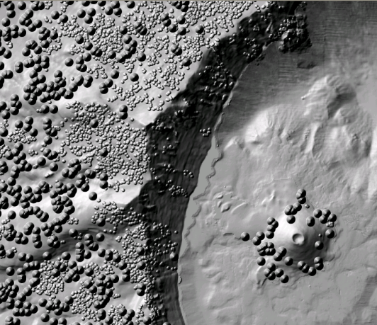
Figure 5. The output from the Bump Map model — in this example, the taller cones represent conifers and the lower domes represent sedge
In our next blog entry, Symbolizing the bump map, we will talk about how you can symbolize the output from the model to create a stunning looking bump map (figure)!
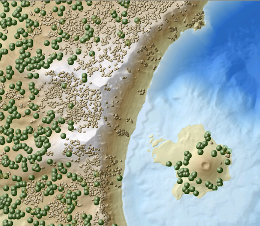
Figure 6. A symbolized bump map
Additional Resources
Presentations:
Buckley, A. and R. Nagi. 2009. “ArcGIS Bump Map Model”, presentation at NACIS PCD 2009 – Sacramento.
Nighbert, J. 2007. “Making Noise with ArcGIS”, presentation at the 27th Esri UC.
Nighbert, J. 2003. “Characterizing Landscapes for Visualization through Bump Mapping and ESRI’s Spatial Analyst”, presentation at the 23rd Esri UC.
Nighbert, J. 2002. “Using ArcGIS to Apply Textures and Materials to Relief Backdrops in Cartographic Presentations”, presentation at the 22nd, Esri UC.
Papers:
Nighbert, Jeffrey. 2003. “Characterizing Landscapes for Visualization Using ArcView Spatial Analyst.” Proceedings of the 23rd Annual Esri User Conference, July 7-11, San Diego, CA.
Nighbert, Jeffrey. 2002. “Using ArcGIS to Apply Textures and Materials to Relief Backdrops in Cartographic Presentations.” Proceedings of the 22nd Annual Esri User Conference, July 8-12, San Diego, CA.
Nighbert, Jeffrey. 2002. “Using Remote Sensing Imagery to Texturize Layer Tinted Relief.” Cartographic Perspectives, Number 36, Spring 2000, pp. 94-96.

Article Discussion: