The results of many geographic analyses depend on the spatial scale of the data and calculations. Surface features vary in size: local features are found with smaller scales while large overarching features may require a larger scale. Multiscale approaches to analysis help you learn about a particular surface and find the optimum scales to characterize its topography. Use the new multiscale tools in ArcGIS Pro 3.4 and 3.5 to explore and better understand the terrain you are working with. These multiscale tools were conceived and developed in consultation with John Lindsay and first appeared in his Whitebox software.
- New in ArcGIS Pro 3.4: the Multiscale Surface Percentile and Multiscale Surface Difference tools
- New in ArcGIS Pro 3.5: the Multiscale Surface Deviation tool
- All these tools will be available in ArcGIS Enterprise in the future

Available parameters
Each of these new tools makes calculations across a range of spatial scales and returns the maximum value for each cell. Here scales are specified through neighborhood distance values. A neighborhood distance is the distance from the target cell center, creating a square of cells around the target cell. To control the scales for analysis, these tools have several optional parameters that identify the minimum and maximum scales and the increment between scales.

Multiscale Surface Percentile and Multiscale Surface Deviation also have a Nonlinearity Factor parameter, which controls the increase in neighborhood distance from the minimum to the maximum. By default, the neighborhood distances will increase linearly, but using the Nonlinearity Factor parameter allows for more customization of the scale sampling distribution. This is advantageous because terrain characteristics are often highly variable at smaller scales and more consistent at larger scales, so these tools give the option to increase sampling density for smaller scales and decrease it for larger scales. For more information on how the Nonlinearity Factor parameter works, visit How Multiscale Surface Percentile works or How Multiscale Surface Deviation works.
In addition, to these analytical parameters, these tools support distributed processing and GPU computation. Using the parallel processing factor environment setting, you can control the number of processors for CPU. Using the Target Device for Analysis parameter, you can select whether the tool will perform calculations on your machine’s CPU or GPU.
Outputs and interpreting results
The primary output for these tools is the statistical value raster, containing the percentile, difference, or deviation value based on the tool run. These values can be taken as indicators of local ruggedness or the presence of features. To support this output, there is also the scale raster, which identifies the scale at which the maximum value was found for each cell. By looking at these rasters together, you can gain valuable insights about your surface’s topographic characteristics. For example, these outputs are used in workflows that extract hydrologic features from a surface.
The following exercise explores the hydrologic features in a landscape. A study area is shown below.

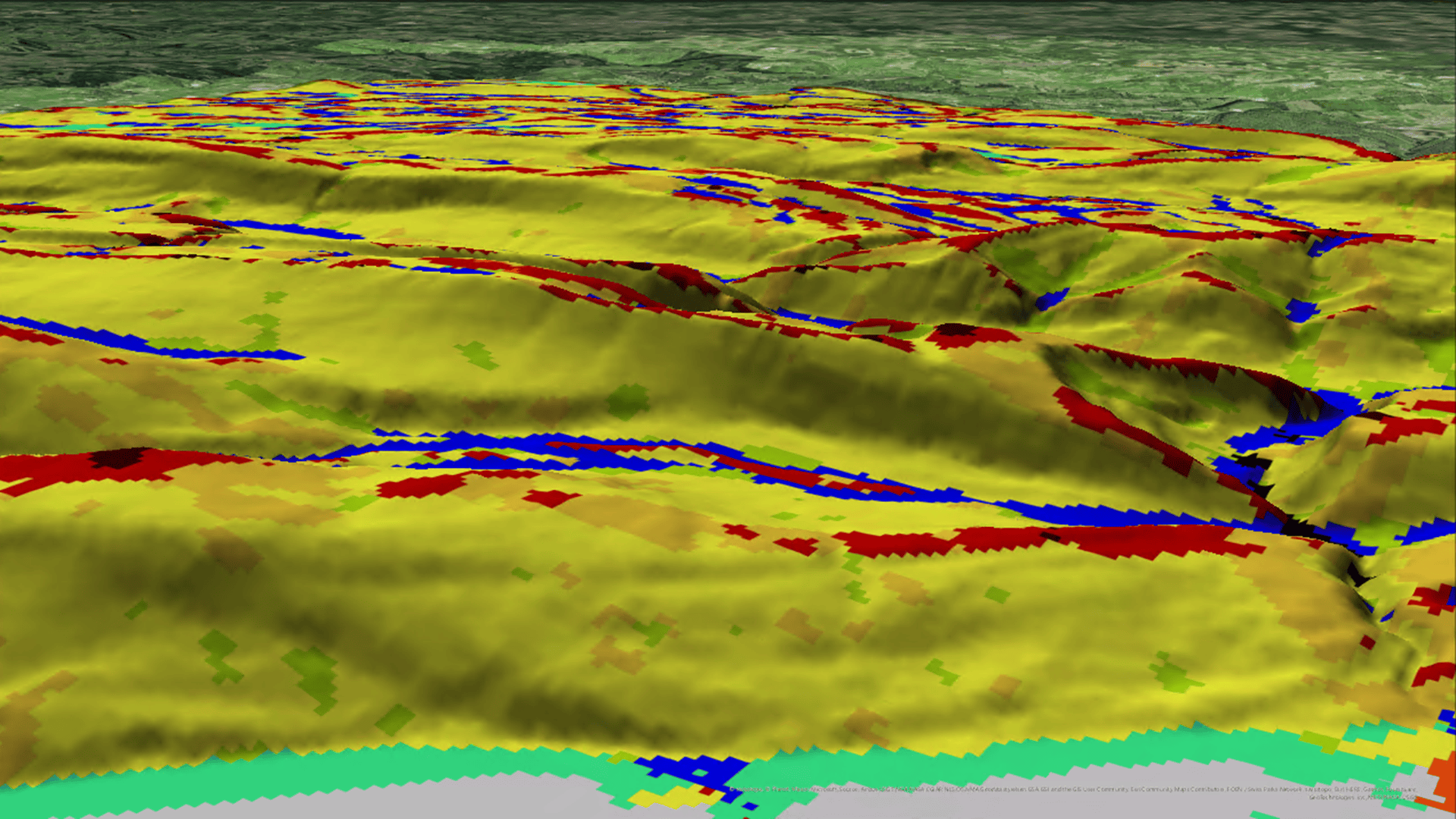
Run the Multiscale Surface Deviation tool with default settings to analyze neighborhood distances from 4 cells to 13 cells with an increment of 1 and a nonlinearity factor of 1. In addition to the primary output, specify the optional output, the scale raster.
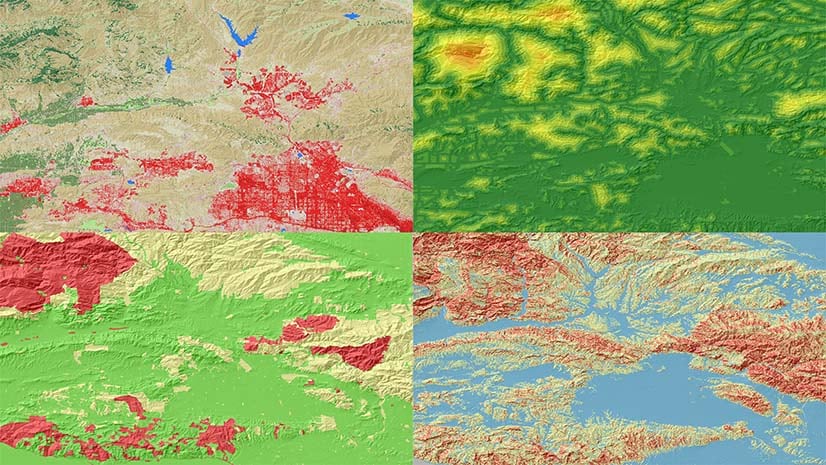
Running with those settings produces the following outputs. Higher positive values tend to occur for local maximums (left, red) in elevation while more negative values (left, blue) appear for local minimums. This means that we are potentially identifying ridges or mountain peaks (local maximums) and flat, valley areas (local minimums). Where we see these negative deviation values, the scale output values tend to be for larger neighborhoods (right, dark green). This means that ridges or peaks and valleys can be identified by finding areas with large neighborhood values and either high positive deviations (ridges, peaks) or high negative deviations (valleys).

Compare these values with output from the Derive Stream As Line tool from the Hydrology toolset. The streams of this study area closely follow the areas where there is a negative deviation value and a large scale. In real-world water applications, this kind of information is used to enhance elevation derived hydrography workflows.

This exercise demonstrated how the Multiscale Surface tools can be used to learn about surface data and the workflows it adds value to. Use these tools in ArcGIS Pro 3.5 with the Surface toolset in the Spatial Analyst toolbox: Multiscale Surface Percentile, Multiscale Surface Difference, and Multiscale Surface Deviation.
Article Discussion: